1. Quantitative results
Validation metrics for each cue detector individually, then for the aggregated segment-level system.
1.1 Parking-sign detection Sign
Final validation results from the best checkpoint after 50 epochs:
| Metric | Value |
|---|---|
| mAP@50 | 0.5487 |
| mAP@50–95 | 0.3824 |
| Precision (box-level) | 0.6616 |
| Recall (box-level) | 0.5373 |
| Best image-level threshold | 0.15 |
| Best image-level F1 | 0.6673 |
| Image-level AUROC | 0.8310 |
Table 1. Main validation results for the parking-sign detector.
The box-level metrics show that the model is learning to localize parking signs reasonably well, while the image-level F1 and AUROC show that it can separate positive and negative images with useful reliability.
1.2 Threshold analysis Sign
We swept the confidence threshold to study the precision-recall trade-off at the image level for the sign detector.
| Threshold | Precision | Recall | F1 | Accuracy |
|---|---|---|---|---|
| 0.15 | 0.6913 | 0.6448 | 0.6673 | 0.9299 |
| 0.20 | 0.7328 | 0.6052 | 0.6629 | 0.9329 |
| 0.30 | 0.7565 | 0.5517 | 0.6381 | 0.9318 |
| 0.50 | 0.8262 | 0.4672 | 0.5969 | 0.9312 |
| 0.70 | 0.9150 | 0.3155 | 0.4692 | 0.9222 |
Table 2. Image-level threshold sweep on the sign-detector validation set.
The best operating threshold is around 0.15. This is relatively low, which indicates that many useful detections are not extremely high-confidence. If a very strict confidence threshold is used, recall drops sharply and many parking cues are lost. This is exactly the kind of behavior that makes aggregation valuable: several weak or partial detections across nearby images may still provide strong segment-level evidence.
1.3 Training progress over time Sign
Key sign-detector checkpoints during training:
| Checkpoint | mAP@50 | Image-level F1 | AUROC |
|---|---|---|---|
| Epoch 20 | 0.4835 | 0.6430 | 0.8088 |
| Epoch 25 | 0.5065 | 0.6535 | 0.8226 |
| Epoch 50 | 0.5487 | 0.6673 | 0.8310 |
Table 3. Progression of sign-detector validation performance across checkpoints.
The model improved steadily throughout training. However, the gains from epoch 25 to epoch 50 were smaller than the gains earlier in training, suggesting that the detector is approaching a plateau. Future gains are more likely to come from aggregation and additional cues than from extensive further tuning of the sign detector alone.
1.4 Zero-shot parking-meter results Meter
In addition to the trained parking-sign baseline, we performed a
preliminary zero-shot experiment for parking-meter detection. We
used a COCO-pretrained YOLO11x detector and
evaluated on the Mapillary Vistas validation split (object--parking-meter
as ground truth):
- 2,000 validation images
- 50 positive images (at least one parking meter)
- 1,950 negative images
Before evaluating on the full validation set, we ran a
positives-only sweep to understand the effect of inference
resolution and confidence threshold. That sweep showed that larger
input resolution substantially improves recall, consistent with the
qualitative observation that parking meters are often very small in
street-view imagery. Based on this analysis we selected
imgsz=1280 for the full run.
| imgsz | conf | Img P | Img R | Img F1 | Box P | Box R | Box F1 |
|---|---|---|---|---|---|---|---|
| 1280 | 0.05 | 0.109 | 0.520 | 0.181 | 0.0469 | 0.168 | 0.0734 |
| 1280 | 0.10 | 0.158 | 0.480 | 0.238 | 0.0758 | 0.158 | 0.1020 |
Table 4. Zero-shot parking-meter evaluation on the Mapillary Vistas validation set using a COCO-pretrained YOLO11x.
For the better setting (imgsz=1280, conf=0.10), the
detailed counts are:
- Image-level: TP = 24, FP = 128, TN = 1822, FN = 26
- Box-level: TP = 15, FP = 183, FN = 80
Three takeaways:
- Zero-shot transfer is real but limited. The detector recovers nearly half of positive parking-meter images at the image level, so it is not behaving randomly.
- Precision is poor. Many false positives, especially on pole-like objects and other narrow vertical street furniture.
- Parking meters are therefore a weak auxiliary cue. Useful in a multi-cue system, but not reliable enough to serve as a primary cue by themselves.
Between the two settings, conf=0.10 gives the better
overall trade-off because it substantially reduces false positives
while only slightly reducing recall — the more reasonable
operating point if parking-meter scores are later incorporated into
cue fusion.
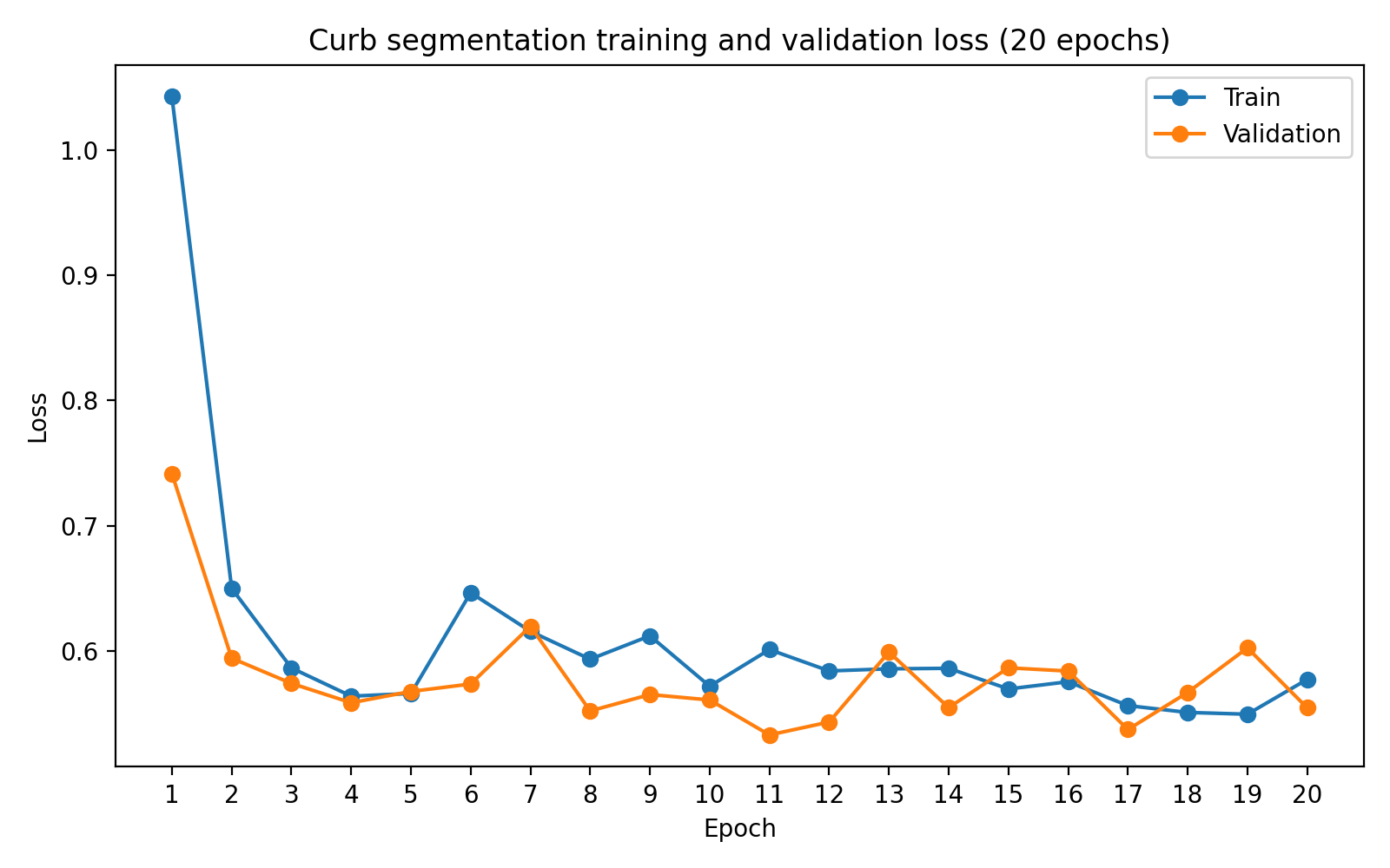
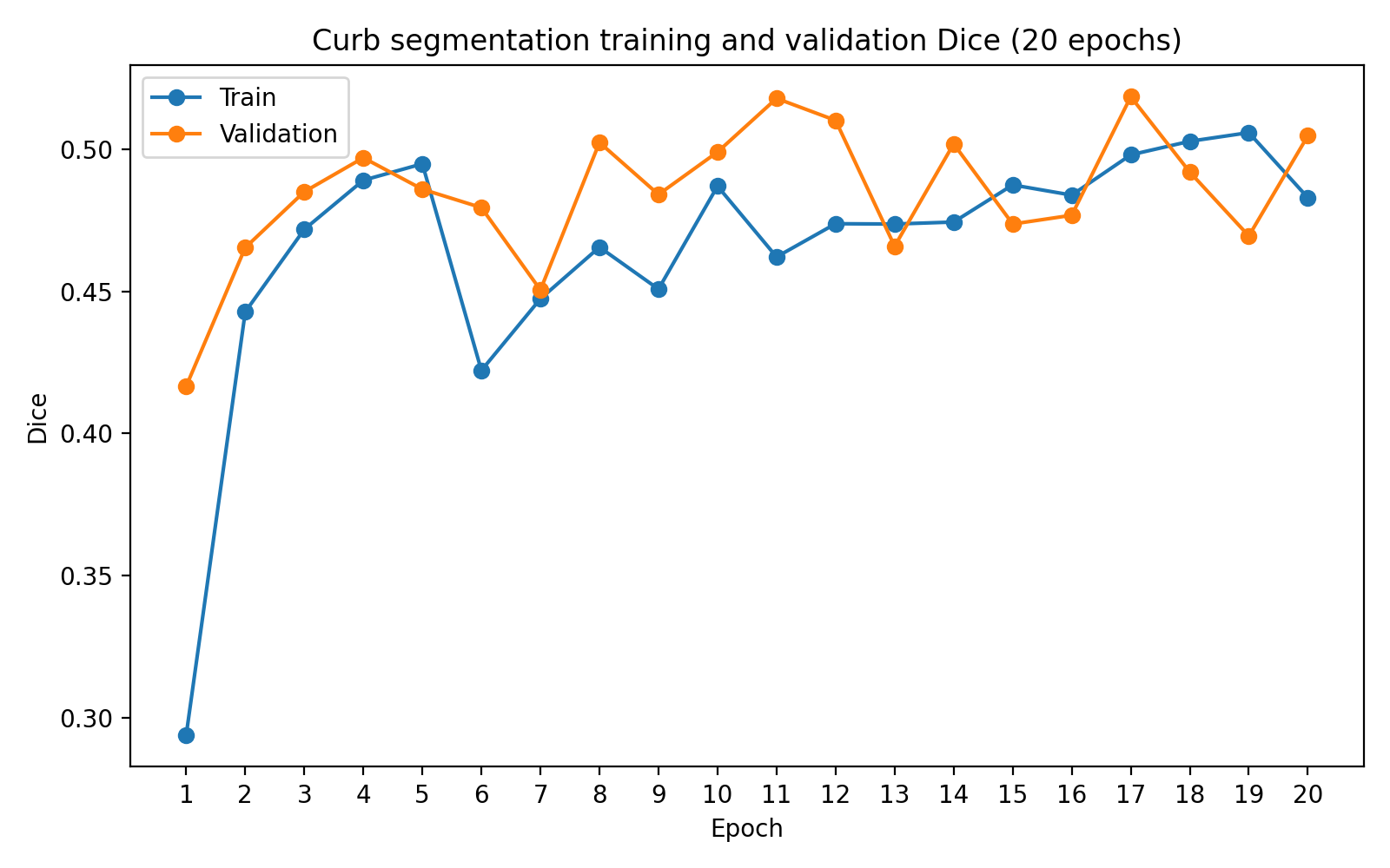
1.5 Curb segmentation and color results Curb
We trained a U-Net curb segmentation model on Mapillary Vistas
(construction--barrier--curb as foreground, binary).
Trained for 20 epochs; best validation checkpoint
at epoch 17:
Several trends are visible in the curves: training and validation losses fall rapidly in the early epochs and then fluctuate within a narrower range; Dice and IoU improve substantially during the first half of training and then plateau; the best validation checkpoint occurs before the final epoch — additional training does not fundamentally change the learned representation. This matches the qualitative observation that the model learns to localize curb boundaries reasonably well, and the remaining errors are largely due to the intrinsic difficulty of thin-structure segmentation rather than undertraining.

Curb-color distribution on the validation set
Using the curb segmentation output, we ran curb color inference on
the 2,000-image validation split. The segmentation model was first
used to predict curb masks, and then an HSV-based color analysis was
applied to the predicted curb boundaries. The final color assignment
was restricted to the set
{red, yellow, green, white, gray, unknown}, with a
conservative fallback to unknown whenever evidence was
weak or ambiguous.
| Dominant color | Count | Fraction |
|---|---|---|
| Unknown | 937 | 46.85% |
| Gray | 835 | 41.75% |
| Yellow | 190 | 9.50% |
| Green | 21 | 1.05% |
| White | 13 | 0.65% |
| Red | 4 | 0.20% |
Table 5. Validation-set distribution of dominant curb-color predictions from the curb-analysis pipeline.
Three conclusions:
- Curb segmentation recovers enough structure for downstream color analysis on a substantial fraction of images, even though the masks are often thin and fragmented.
- Strong painted curb colors are sparse. Gray and unknown dominate, consistent with most curbs being unpainted, weakly painted, or visually ambiguous.
- Conservative uncertainty handling is necessary — forcing a hard color in every case would introduce many incorrect labels.
An earlier version of the color pipeline used all predicted mask pixels for color extraction. That approach produced noticeably more contamination from nearby white road markings and crosswalks. After switching to boundary-based color extraction, the number of white predictions dropped substantially while gray became more common, suggesting the revised pipeline more accurately captures curb surface color rather than nearby painted road elements. Some recall is traded for better precision and interpretability.
1.6 Segment-level synthetic aggregation Aggregation
The segment-level aggregation experiment is the main system-level result of the project. The synthetic pseudo-segment benchmark contains 225 five-image segments: 80 negative segments and 145 positive segments. Positive segments were constructed to include at least one parking-related cue, while negative segments contained no selected strong cue. The construction tests whether a segment-level rule can recover sparse evidence distributed across multiple views.
Final cue-pool sizes used to build this dataset:
- Sign-positive images: 4,446
- Meter-positive images: 50
- Strong curb-color images: 228
- None / neutral images: 41,185
The meter pool is especially small. This directly shaped the final segment distribution — we reduced meter-heavy segment types to avoid reusing the same meter examples too frequently. Repeated reuse would make the evaluation less diverse and would overstate the amount of meter evidence available in the data.
| Segment type | Number | Label |
|---|---|---|
| None | 80 | 0 |
| Sign only | 50 | 1 |
| Meter only | 15 | 1 |
| Curb color only | 25 | 1 |
| Sign + meter | 15 | 1 |
| Sign + curb color | 20 | 1 |
| Meter + curb color | 10 | 1 |
| Sign + meter + curb color | 10 | 1 |
| Total | 225 | — |
Table 6. Final synthetic pseudo-segment distribution. Each segment contains five images. The skew reflects cue sparsity, with more negative and sign-only segments and fewer meter-heavy combinations.
The synthetic dataset should be interpreted with the correct scope. It does not claim that randomly combined images are actual road-neighboring views. It is a controlled multiple-instance benchmark for the aggregation mechanism — useful because it isolates a key property of the task: a segment may be positive even if only one of several views contains visible evidence.
Aggregation vs. single-image baseline
The baseline uses one selected image from each segment and applies only the sign score. This simulates a single-view deployment setting. The aggregation method uses all five images and combines sign, meter, and curb evidence using the weighted-max rule described in Approach › Segment-level aggregation.
| Method | Threshold | Precision | Recall | F1 |
|---|---|---|---|---|
| Single-image baseline | 0.05 | 0.784 | 0.200 | 0.319 |
| Segment aggregation | 0.15 | 0.753 | 0.924 | 0.830 |
Table 7. Synthetic pseudo-segment aggregation results. Aggregation substantially improves recall and F1 compared with a single-image per-segment baseline.
The result is strong and directly supports the project hypothesis. The single-image baseline has high precision but extremely low recall: when it detects a sign the prediction is meaningful, but it misses most positive segments because the selected view often lacks visible evidence. Aggregation makes the opposite trade-off — precision drops only slightly (0.784 → 0.753), but recall rises from 0.200 to 0.924. Aggregation is mainly solving the false-negative problem caused by sparse cue visibility. Precision decreases slightly because aggregation treats any strong cue from any view as sufficient evidence, which increases true positives but also lets in some false positives from noisy auxiliary cues such as meters and curb color.
Threshold sweep on the aggregated score
| Threshold | Precision | Recall | F1 | AUROC |
|---|---|---|---|---|
| 0.05 | 0.671 | 0.972 | 0.794 | 0.820 |
| 0.10 | 0.711 | 0.966 | 0.819 | 0.820 |
| 0.15 | 0.753 | 0.924 | 0.830 | 0.820 |
| 0.20 | 0.774 | 0.876 | 0.822 | 0.820 |
| 0.25 | 0.800 | 0.800 | 0.800 | 0.820 |
| 0.30 | 0.823 | 0.738 | 0.778 | 0.820 |
| 0.40 | 0.878 | 0.545 | 0.672 | 0.820 |
| 0.50 | 0.946 | 0.483 | 0.639 | 0.820 |
Table 8. Threshold sweep for the synthetic segment-level aggregation score. Best F1 at threshold 0.15.
Best F1 occurs at threshold 0.15, the same general operating region as the image-level sign detector. This reinforces the observation that low-confidence detections should not be discarded too aggressively — in this task, weak cues become reliable when pooled over several views.
The practical interpretation is that segment-level aggregation is not merely a post-processing trick. It changes the operating regime of the system. Single-image inference asks each view to independently contain enough evidence; aggregation lets the system use the best available evidence from the local context. This is much closer to the real-world structure of the task.
1.7 Manual real-world segment scores Aggregation
To test whether the same behavior appears outside the synthetic pseudo-segment setting, we manually collected a small real-world dataset of six street segments, each containing five nearby views from the same local curbside context (Google Maps / Street View-style imagery). Only 30 images total — not a statistically significant benchmark, but a useful qualitative validation.
Manual construction is expensive: each segment requires identifying a street with visible parking-related evidence, moving through nearby views, saving images consistently, ensuring the views correspond to the same local curbside context, and writing notes about which cues are visible. We therefore collected six examples covering different cue configurations rather than attempting to build a large benchmark.
| Segment | Label | Observed cue pattern |
|---|---|---|
| seg_000 | Positive | Multiple parking signs visible across the five views, including a faint sign in one view. Tests whether aggregation increases confidence when the sign detector already has evidence. |
| seg_001 | Positive | Meter-only segment. Parking meters in a subset of views; sign evidence absent. Tests whether the meter cue can rescue a segment missed by a sign-only baseline. |
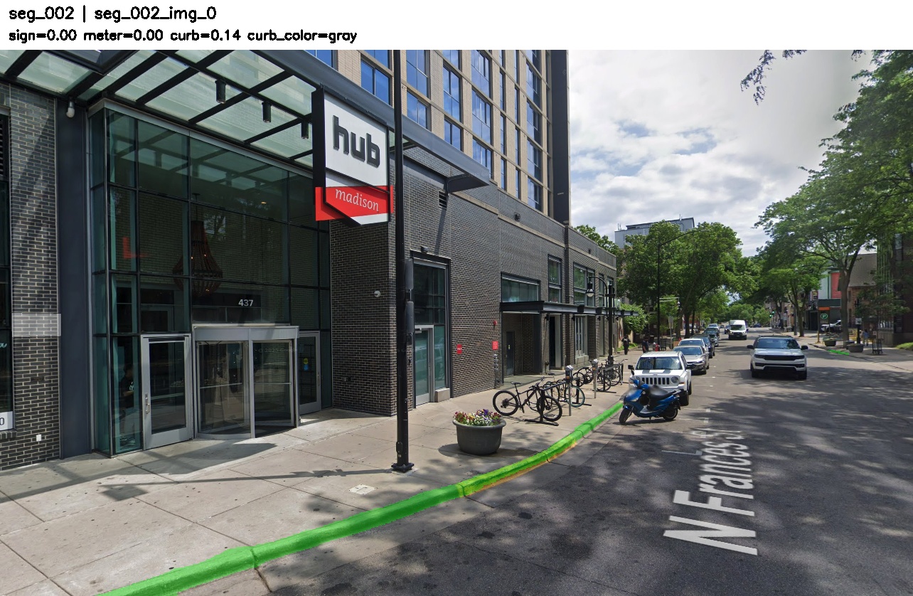
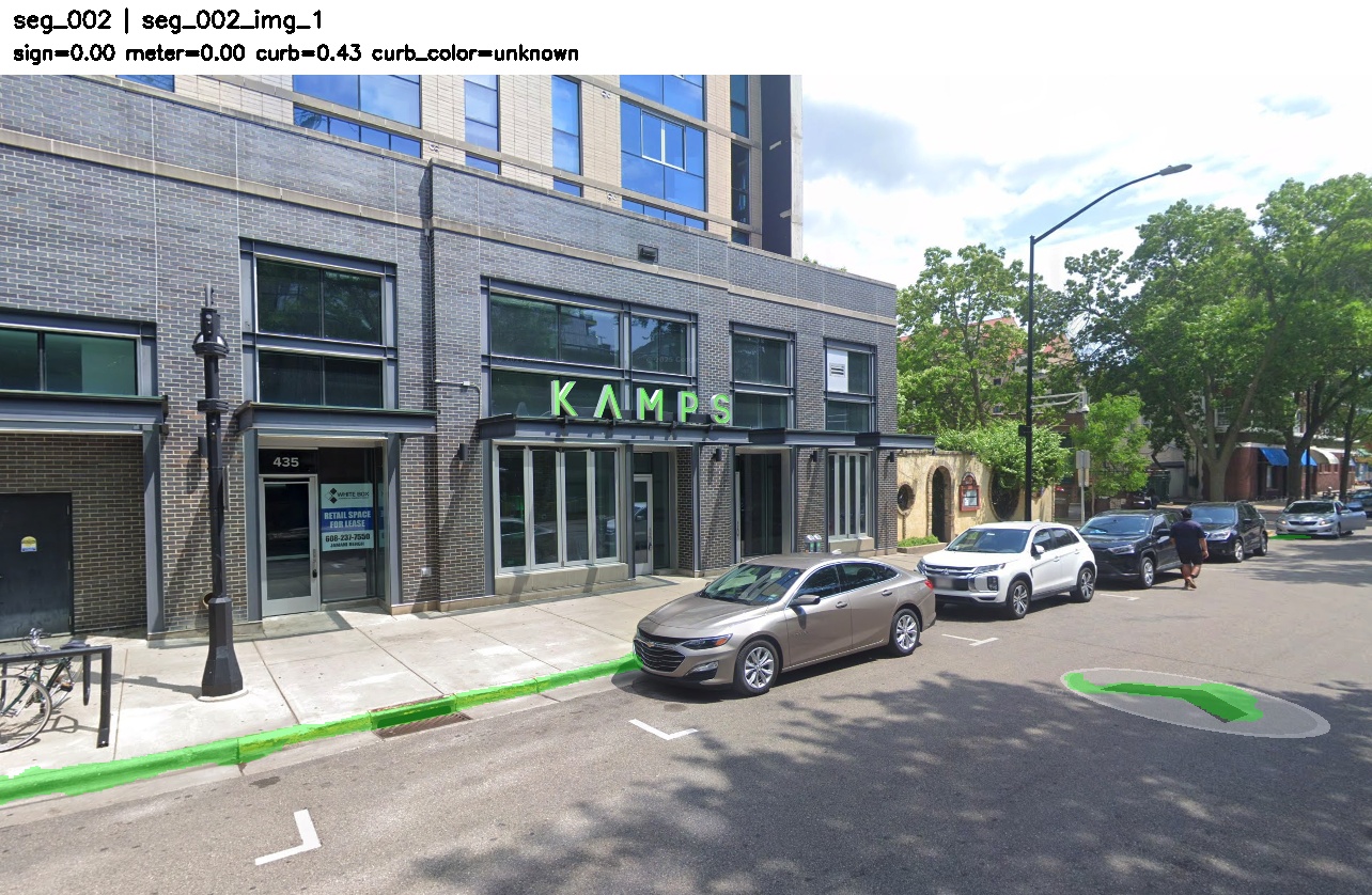
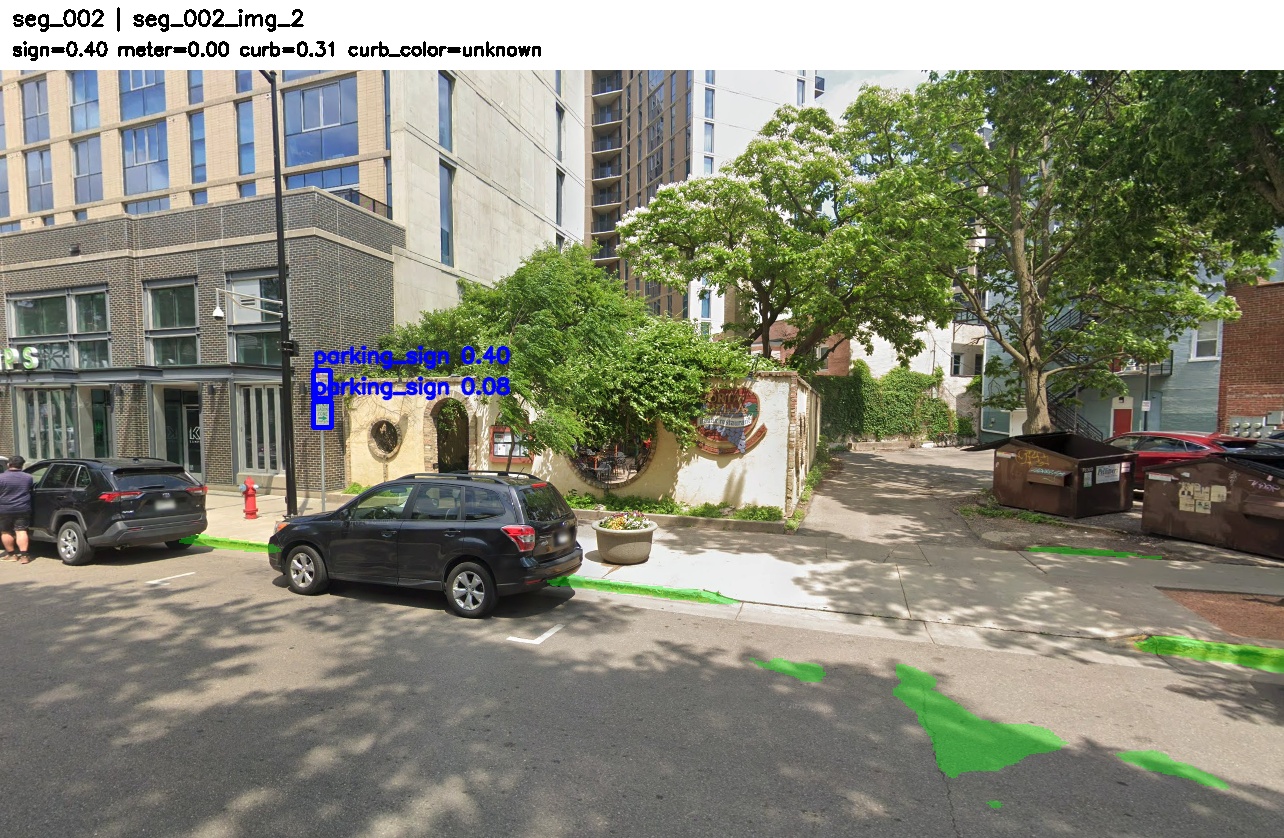
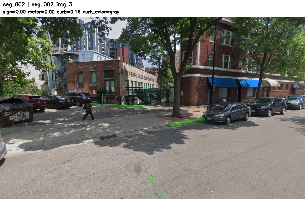
| seg_002 | Positive | Mixed-cue segment containing parking meter, parking-sign evidence, and yellow curb color. Tests whether heterogeneous cues support the same segment-level decision. |
| seg_003 | Positive | Yellow curb-color-only segment. Weak-cue case — no strong sign or meter evidence. |
| seg_004 | Positive | Yellow curb color plus one visible parking meter. Tests complementary cue fusion between meter and curb evidence. |
| seg_005 | Positive | Difficult failure case. Visible sign is not part of the detector's training distribution and resembles a non-standard / storefront sign more than the mapped MTSD parking-sign classes. |
Table 9. Manually collected real-world segment examples.
| Segment | Single | Sign max | Meter max | Curb max | Combined | Pred. |
|---|---|---|---|---|---|---|
| seg_000 | 0.431 | 0.529 | 0.394 | 0.634 | 0.529 | 1 |
| seg_001 | 0.000 | 0.000 | 0.722 | 0.359 | 0.433 | 1 |
| seg_002 | 0.000 | 0.395 | 0.227 | 0.426 | 0.395 | 1 |
| seg_003 | 0.000 | 0.148 | 0.000 | 0.407 | 0.163 | 1 |
| seg_004 | 0.000 | 0.000 | 0.708 | 0.539 | 0.425 | 1 |
| seg_005 | 0.000 | 0.000 | 0.000 | 0.093 | 0.037 | 0 |
Table 10. Manual real-world segment results. Scores are maximum segment-level cue scores. The combined score uses the same weighted-max rule as the synthetic experiment.
Aggregation correctly identifies five of six positive examples; the single-image sign baseline only succeeds on seg_000. Aggregation improves recall by allowing evidence to come from any view and from auxiliary cues.
The annotated views for each segment — with overlaid sign boxes, meter boxes, and curb mask — are gathered in Section 4 below.
2. Validation plots
Standard YOLO validation curves and confusion matrices for the parking-sign detector.
2.1 Detection curves Sign
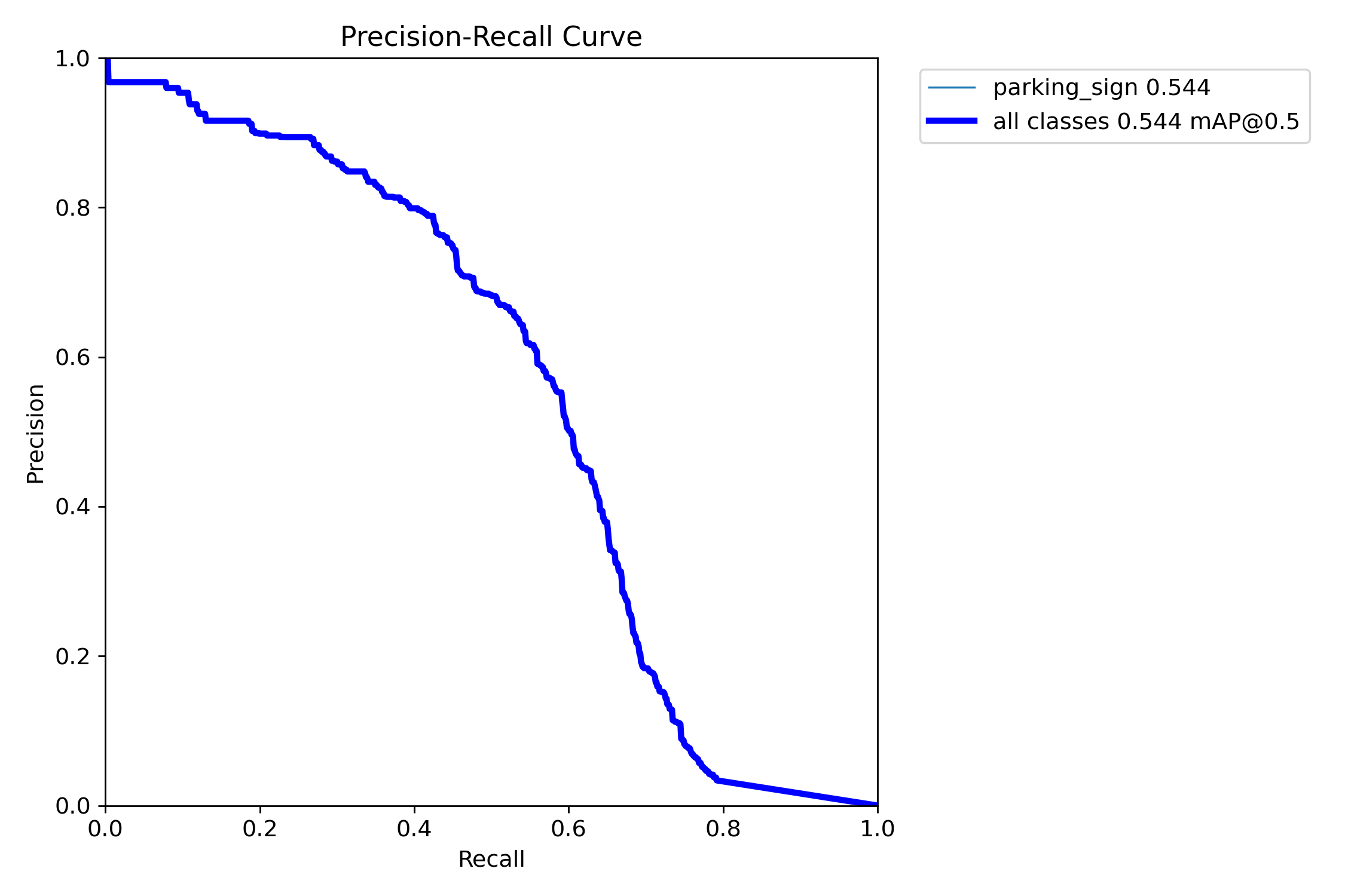
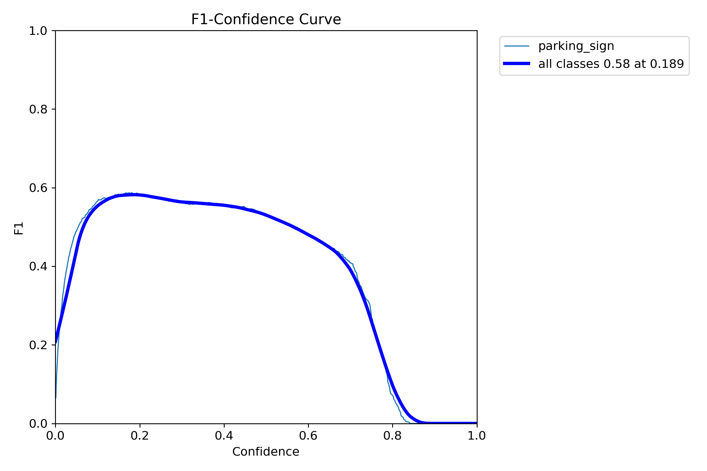
Two takeaways:
- The precision–recall curve confirms moderate but useful detection performance, with mAP@50 around 0.54.
- The F1–confidence curve shows that the detector works best at a relatively low confidence threshold — retaining weaker detections matters.
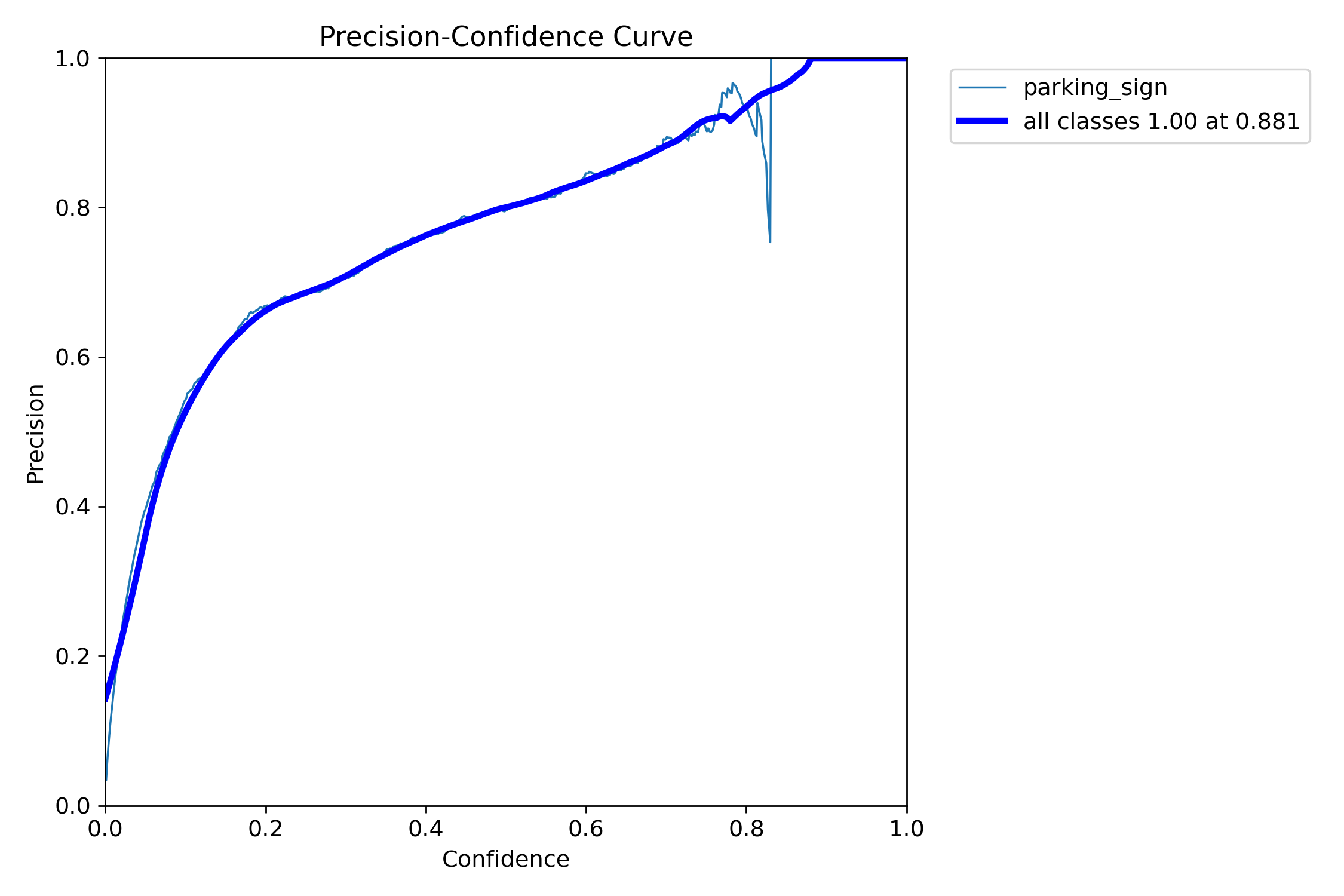
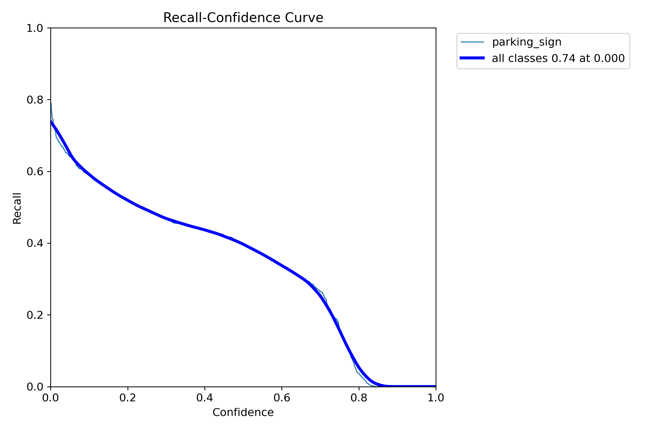
Precision rises with stricter thresholds, but recall drops rapidly — another sign that strict single-image decision rules are not ideal for this task.
2.2 Confusion matrices Sign
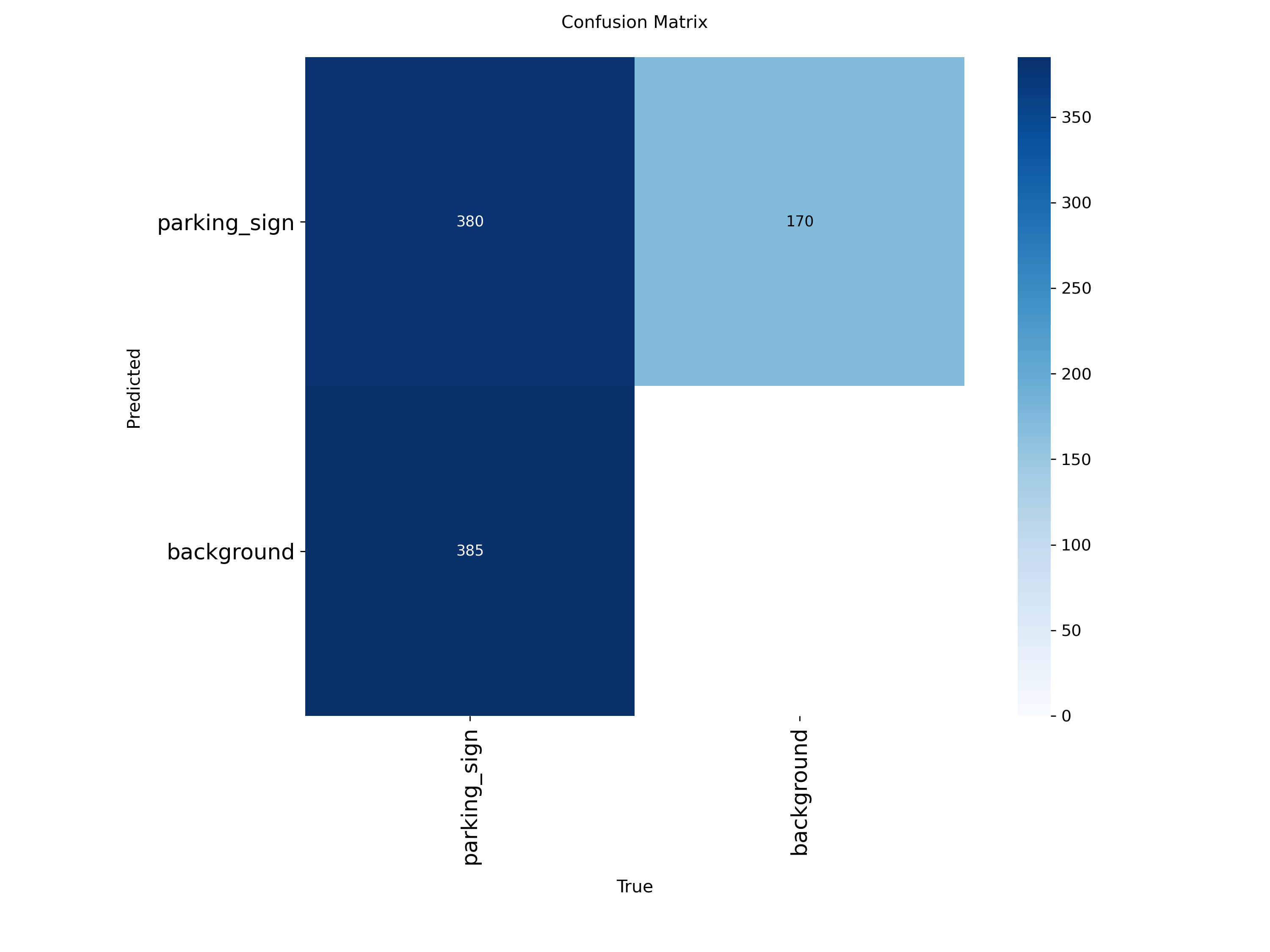
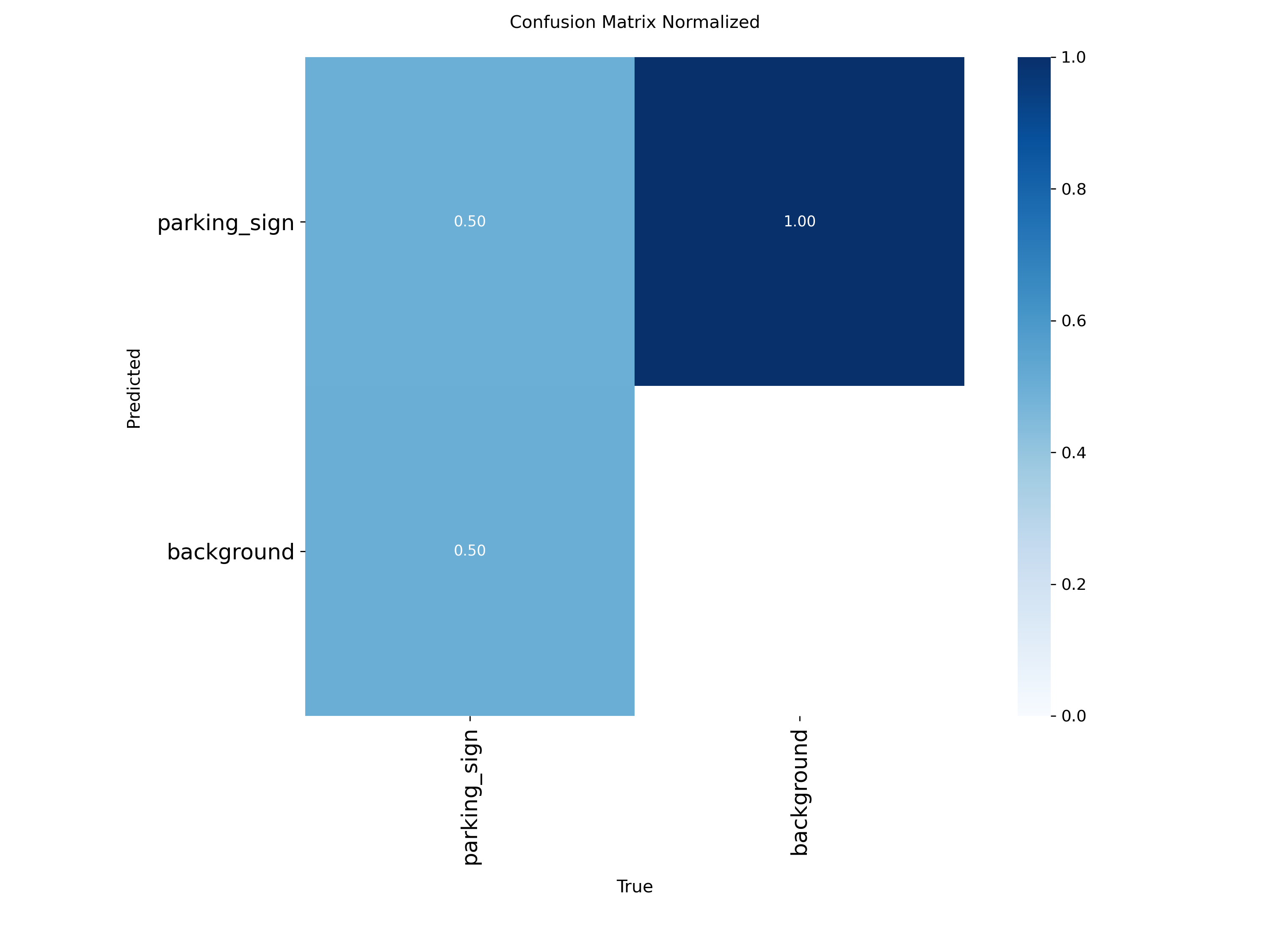
The detector still produces a meaningful number of false negatives, consistent with the moderate recall values reported above. Future gains are unlikely to come only from tightening the detector threshold — combining evidence across views is the more promising direction.
3. Qualitative findings & error analysis
A useful part of the project is not just the final numbers, but the qualitative analysis of why the models succeed or fail. This section walks through the most informative successes and failures cue-by-cue.
3.1 Resolution and scale sensitivity for parking signs Sign
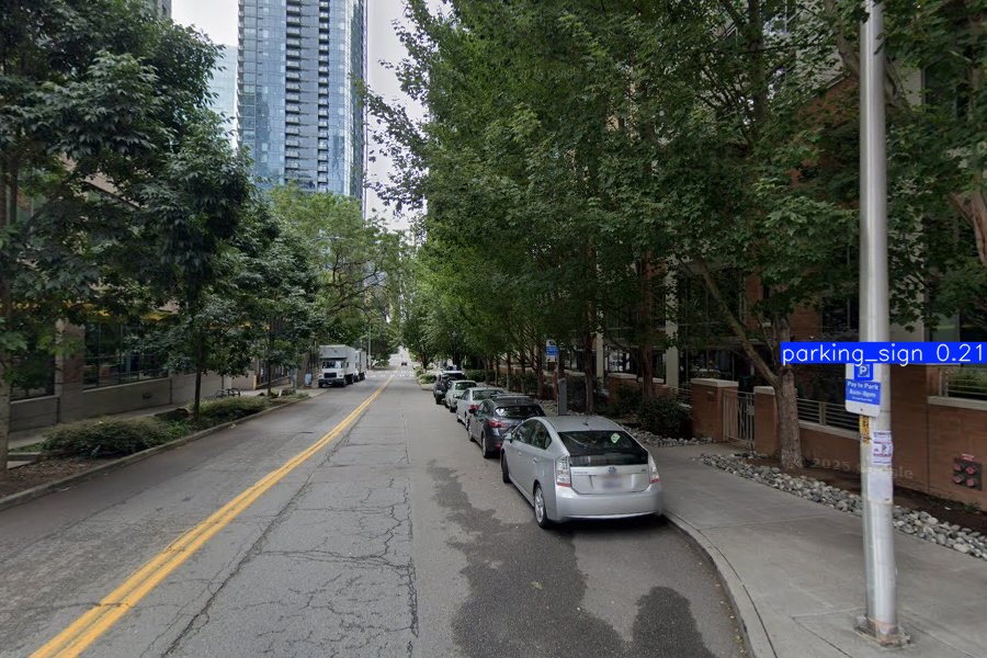
One of the clearest findings: the parking-sign detector is strongly limited by object scale. We tested the same scene at different effective scales:
- At imgsz=640 on the zoomed-out image, the model missed both parking signs.
- At imgsz=960, the model detected one of the signs.
- At imgsz=1280, the model detected both signs.
- On a manually zoomed-in crop, the model detected the signs reliably even at imgsz=640.
This is a strong confirmation of the dataset analysis: the detector is resolution-limited rather than concept-limited. The model has learned what parking signs look like; in wide street scenes, signs are simply too small after image resizing for reliable detection.
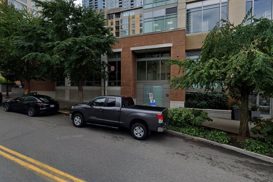
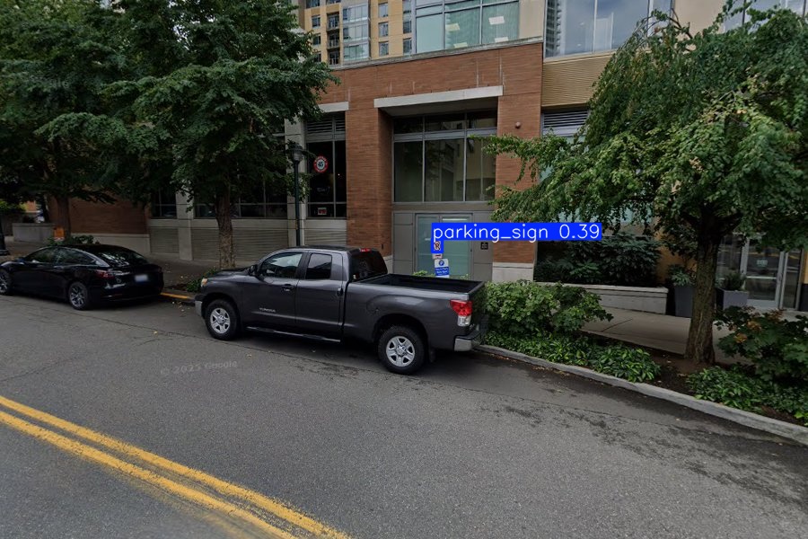
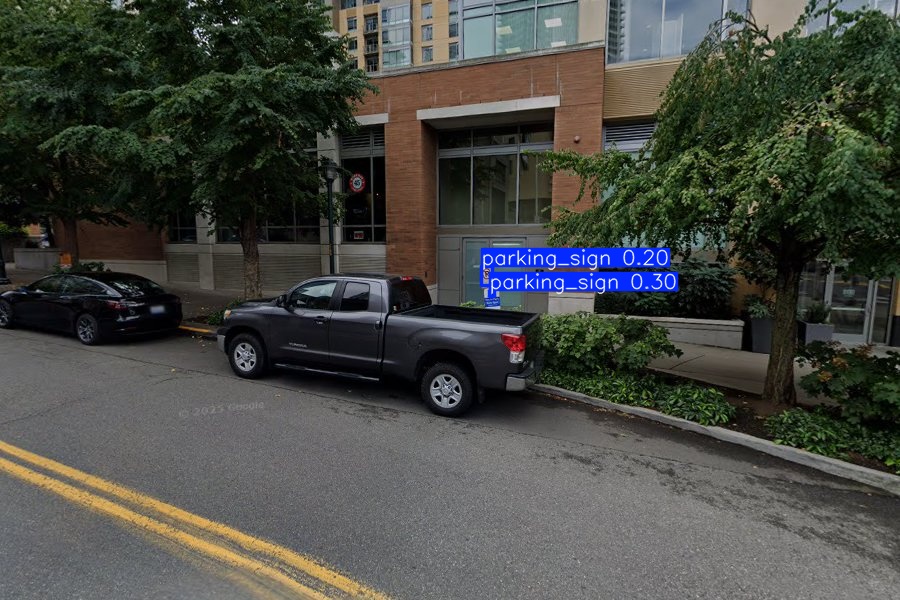
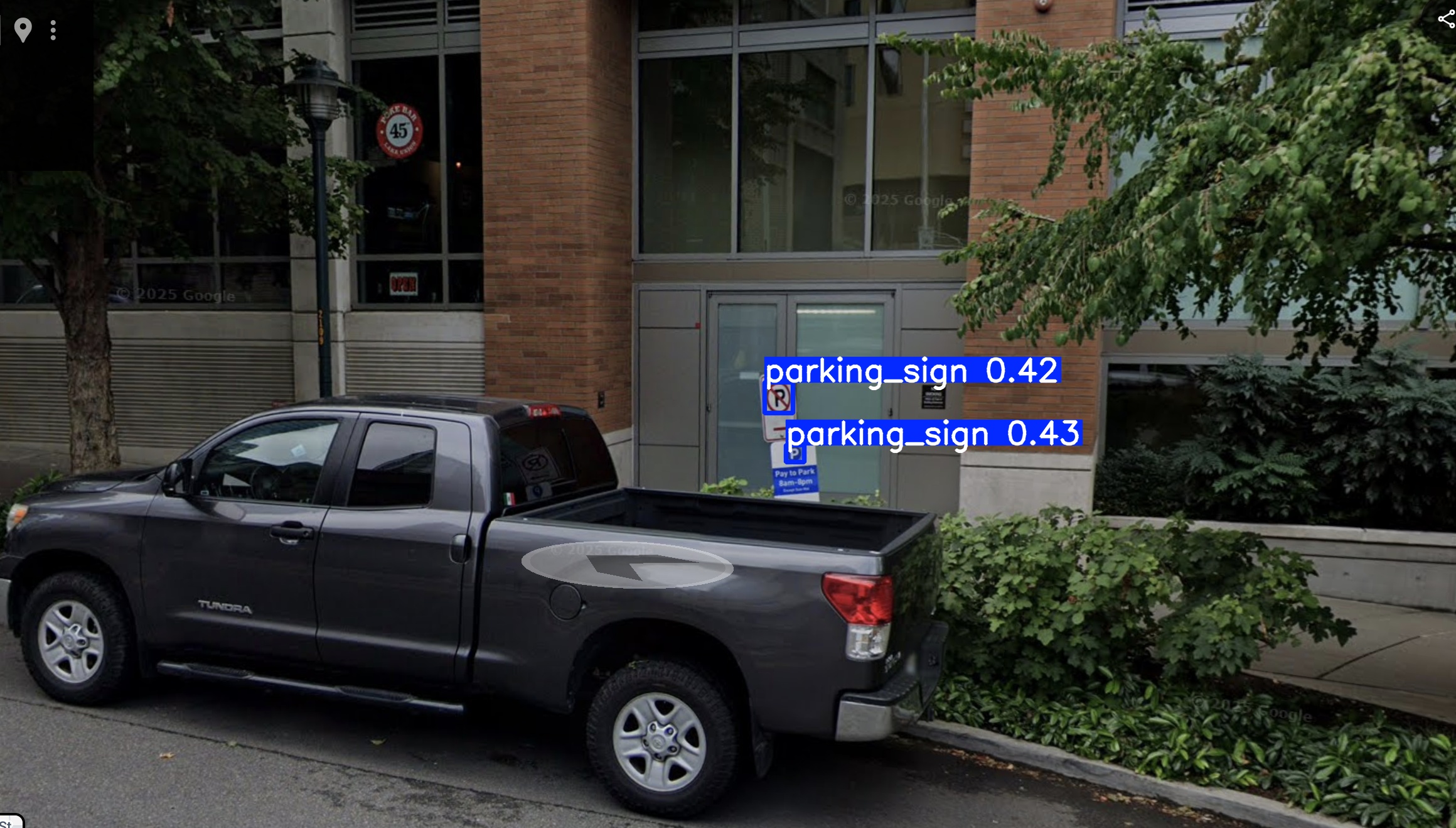
Detection results for a Seattle scene at different effective scales. Detection improves as the parking signs occupy more pixels in the model input. Click any image to step through them in a slideshow.
This finding directly supports the project motivation. If a single view is zoomed out, the cue may be missed; if another nearby view captures the sign more closely, the cue may become detectable.
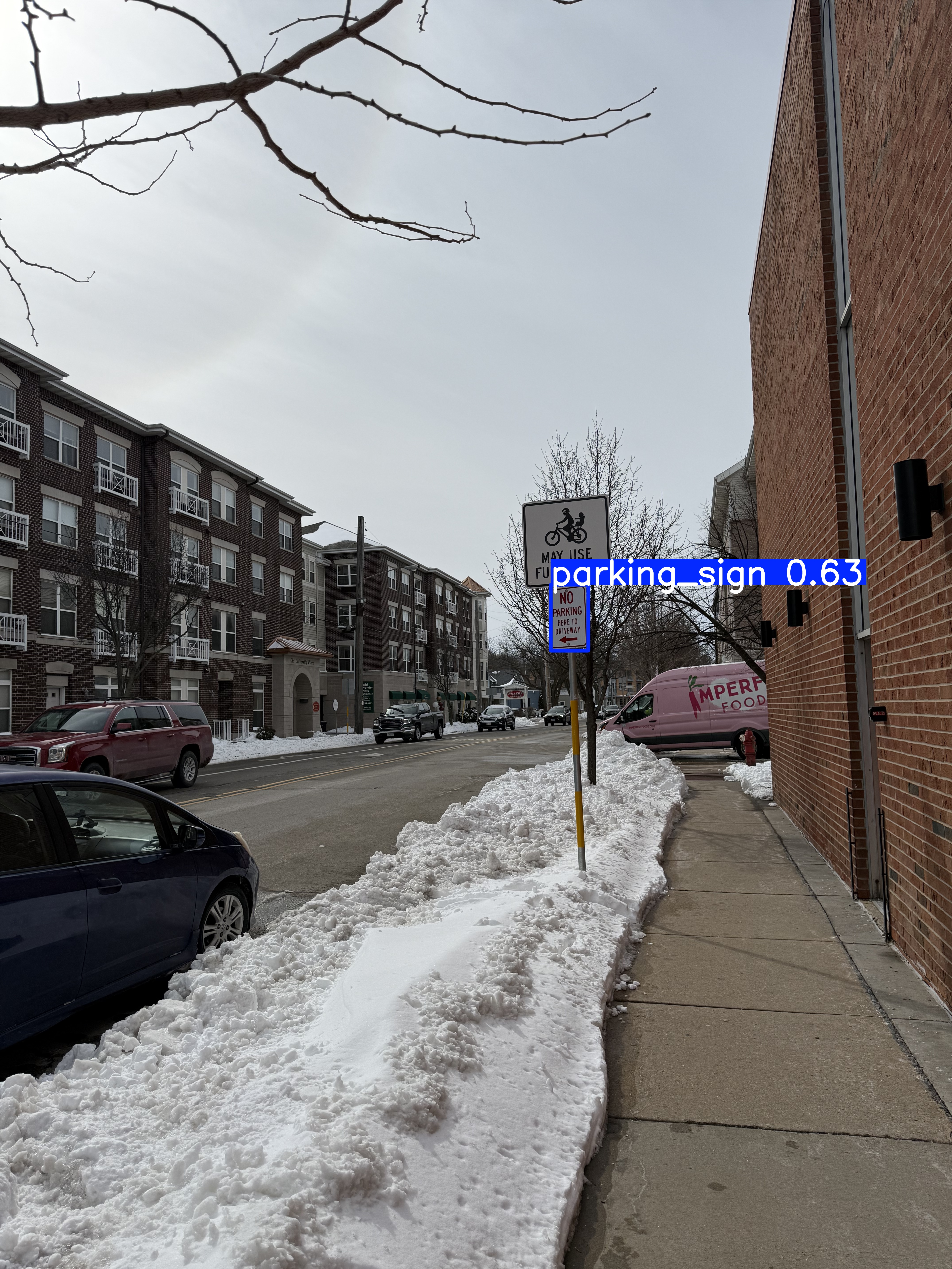
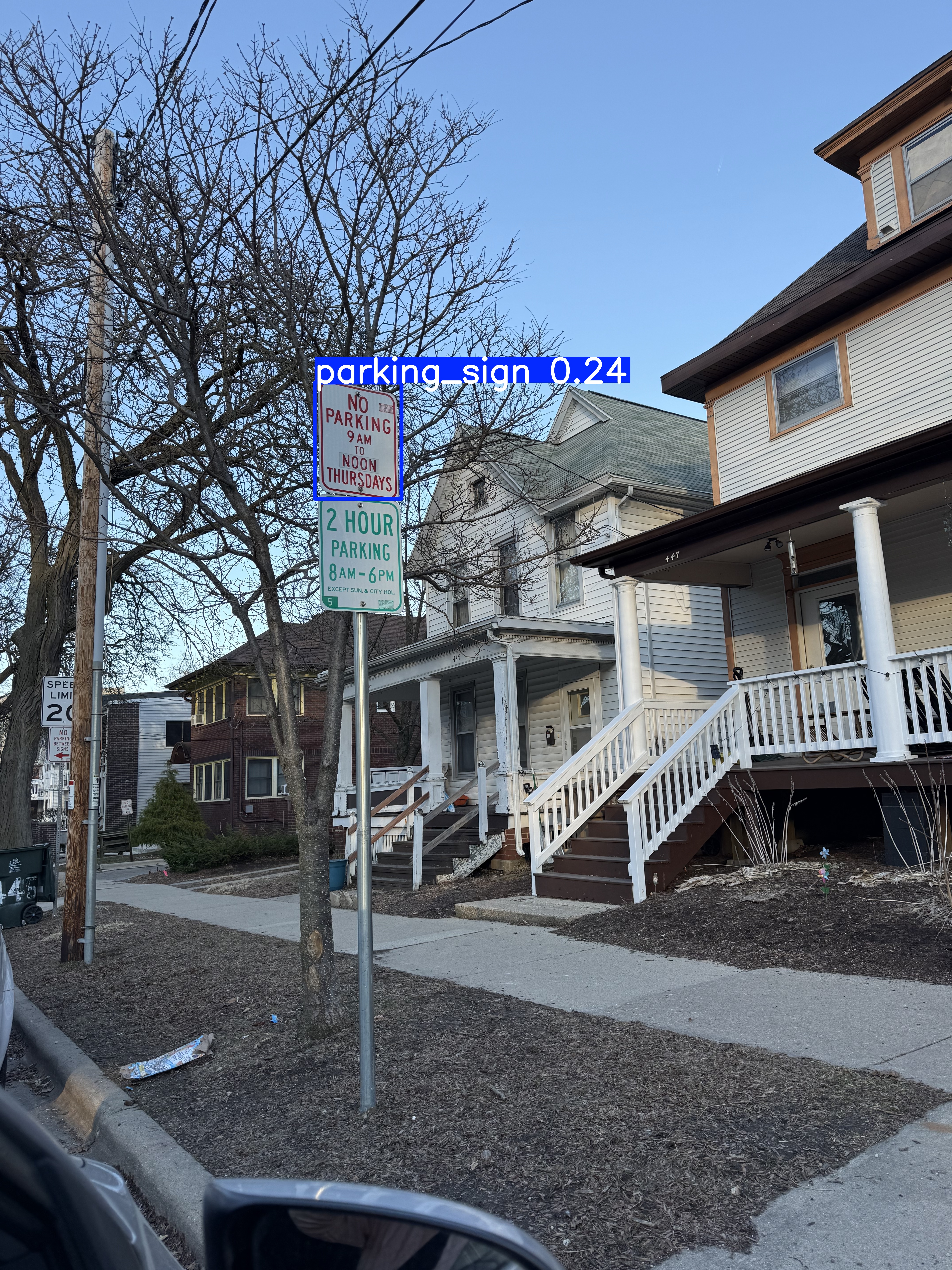
3.2 Partial localization of composite signs Sign
The detector often boxes only the most salient sub-part of a parking-sign assembly — the blue "P" symbol or a no-parking icon — rather than the full stacked signboard including time restrictions.
- MTSD is a traffic-sign dataset, so annotations are naturally sign-centric rather than designed for full sign-assembly understanding.
- Text-heavy restriction plates are smaller and more variable than the main symbol panel, making them much harder to learn.
For the present task this is acceptable because the requirement is parking-cue presence detection, not full OCR-based rule parsing. It is, however, a clear limitation: the detector is suitable for cue detection but not yet for complete parking-rule understanding.
3.3 The non-intuitive small-image case Sign
During qualitative evaluation we observed a non-intuitive behavior: in certain cases, reducing the input resolution (e.g. from 640 to 160) improved the detection of distant parking signs.
YOLO operates on fixed-size inputs and relies on hierarchical feature maps for multi-scale detection, so detection performance is strongly tied to the relative size of the object within the resized image. At higher resolutions, distant parking signs occupy only a small number of pixels relative to the full image; after multiple downsampling operations they become extremely small in deep feature maps. When the input is resized to a smaller resolution, the background is compressed and the object occupies a larger relative portion of the image — effectively boosting its prominence in deeper feature maps, making detection easier.
This is consistent with the dataset analysis: many parking signs in the training data are small and low-resolution, especially in wide street-view images. The model learns to detect parking signs at specific relative scales, which makes detection sensitive to object scale and image resolution. Practical implications:
- Detection performance is sensitive to object scale and image resolution.
- Text-heavy signs are particularly affected due to their dependence on fine-grained visual details.
- A single fixed input resolution may not be sufficient for robust detection across all scenarios.
To address these limitations, several improvements are natural to consider:
- Higher-resolution inference (e.g. 960 or 1280) to better capture small objects.
- Multi-scale inference to improve robustness across object sizes.
- Tiled or patch-based inference for better small-object detection.
- OCR-based methods in future work for better handling of text-heavy parking signs.
Overall, this experiment highlights the importance of object scale in detection performance and provides valuable insight into the limitations of purely visual detection approaches for parking-sign understanding.
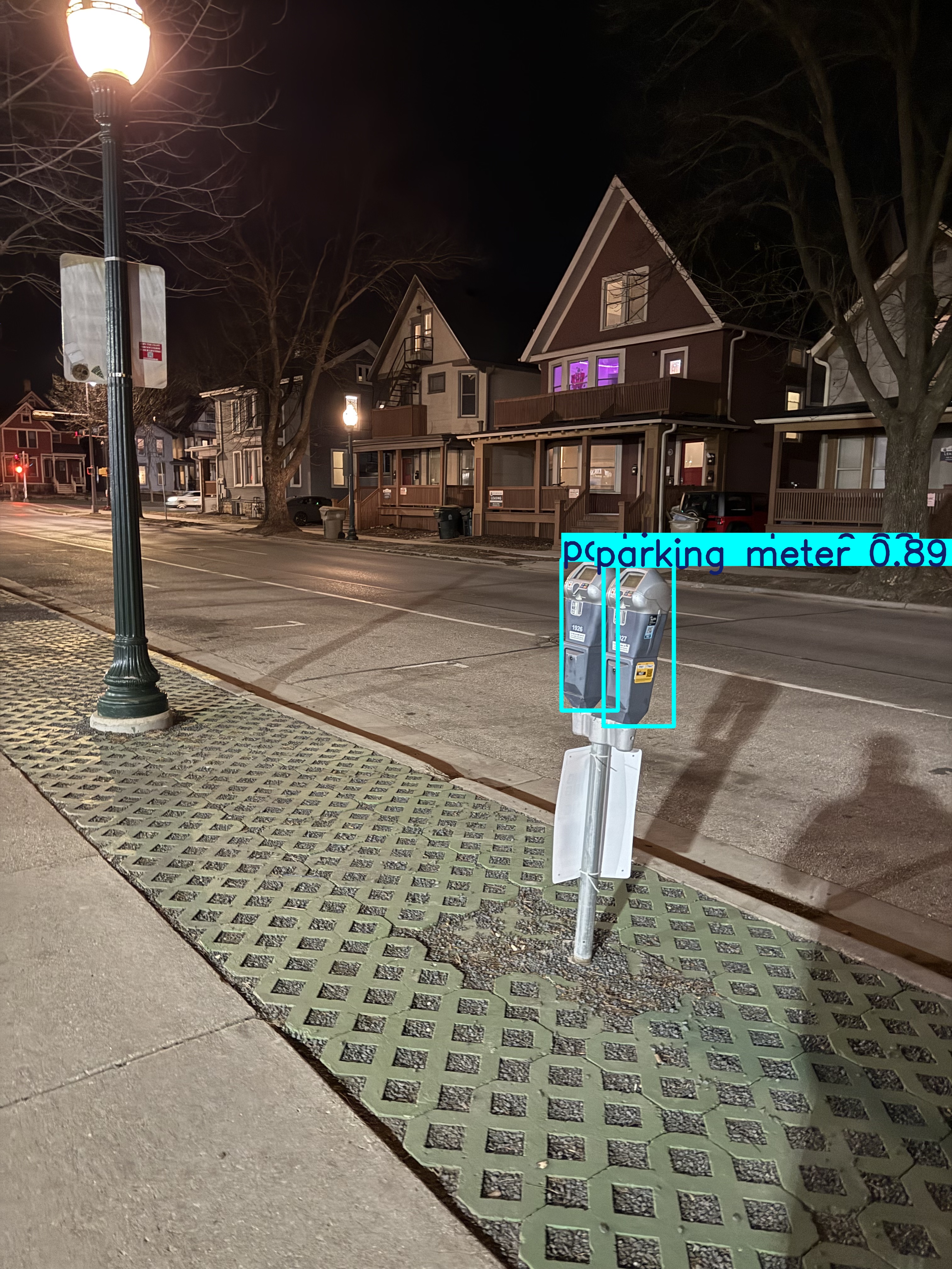
3.4 Qualitative parking-meter findings Meter
On close, clear images, the COCO-pretrained detector can correctly identify parking meters. In realistic street-view scenes — meters small relative to the full image, partially occluded, or visually similar to signposts and other narrow vertical street furniture — the model struggles much more.
This behavior matches the quantitative results: image-level recall shows transferable signal, but low precision indicates the model frequently mistakes pole-like objects for parking meters. Taken together, qualitative meter results match the quantitative findings: parking-meter detection is useful as a partial cue, but currently too noisy to be relied on by itself.
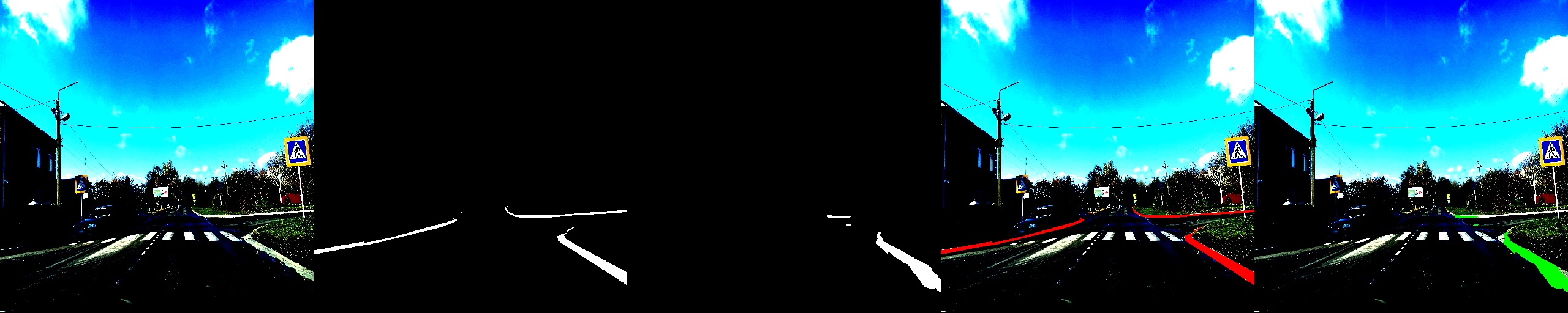
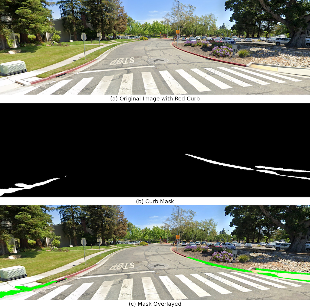
3.5 Qualitative curb segmentation findings Curb
The curb segmentation model produces a useful but imperfect signal. In many scenes it correctly identifies the curb boundary and captures enough structure for downstream analysis. Unlike parking signs or meters, curb regions are long, thin, and often visually weak — predicted masks are frequently sparse and fragmented rather than dense, continuous regions. This is not necessarily a failure for our use case; since the downstream goal is to recover a coarse curb-related cue rather than a pixel-perfect geometric model, even partial mask recovery can be sufficient if the predicted pixels are located on the true curb boundary.
The model exhibits a recurring failure mode on painted or low-elevation curbs, which can look visually similar to flat road paint or lane markings rather than a structurally distinct boundary. The model relies strongly on geometric and shading cues and is less robust when the curb is visually smooth, uniformly painted, or weakly separated from adjacent surfaces.
The painted-curb failure shown below is missed because it lacks strong geometric separation from the road surface. This is likely influenced by dataset bias: many training examples emphasize raised curbs with clear boundary structure. As a result the model relies heavily on geometric edge cues rather than learning a fully semantic notion of curb appearance. When the curb is flat, painted, or visually similar to road markings — especially in zoomed-in views where contextual cues are reduced — the model struggles to distinguish it from surrounding surfaces.
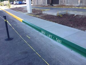
3.6 Qualitative curb color findings Curb
The curb color stage produced some of the most informative
qualitative findings. A straightforward initial approach —
classifying color using all pixels inside the predicted curb mask
— led to substantial contamination from nearby structures such
as crosswalk stripes, painted road markings, and adjacent asphalt.
White road markings in particular caused the system to over-predict
white even when the curb itself was not white.
To address this, we changed the pipeline to use boundary-based color extraction. Instead of taking all predicted mask pixels, we compute the edges of the predicted curb mask and use only those boundary pixels for HSV-based color analysis. This significantly reduces contamination from nearby structures such as crosswalk markings and lane paint, and produces more conservative but more reliable curb-color predictions.
We also found that color prediction requires explicit
uncertainty handling. In many realistic scenes, the
curb mask contains a mixture of red curb paint, white crosswalk
markings, gray asphalt, and lighting variation; the color
distribution becomes multi-modal rather than dominated by a single
class. Instead of forcing a hard label, we introduced a
confidence-margin rule: a color is accepted only if it has both
sufficient absolute confidence and a sufficient margin over the
second-best color. Otherwise, the prediction is labeled
unknown. This made the final output more conservative,
but also more trustworthy.
unknown rather than forcing an incorrect dominant
color — a useful project-level lesson: for curb color,
precision matters more than forcing coverage.
4. Annotated real-world segments Aggregation
Annotated outputs from the manual segment visualization script. Each segment is shown as multiple nearby views with overlaid detections for parking signs, parking meters, and the curb segmentation mask. Click any image to open the slideshow — use the arrow buttons or ← / → keys to step through the five views in a single segment.
4.1 seg_001 — meter-only success
Sign 0.000, Meter 0.722, Curb 0.359 → Combined 0.433. The sign detector contributes nothing; the parking-meter cue is strong enough that aggregation correctly classifies the segment as positive after the 0.6 down-weighting.
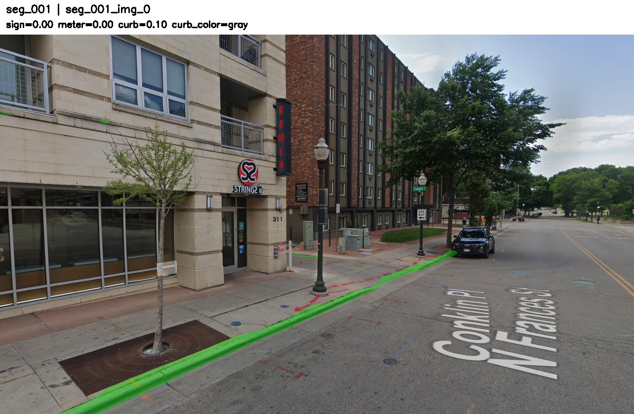
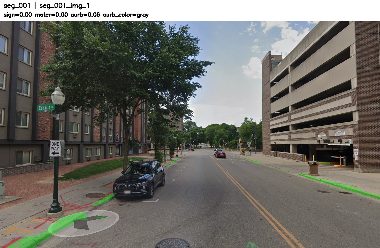
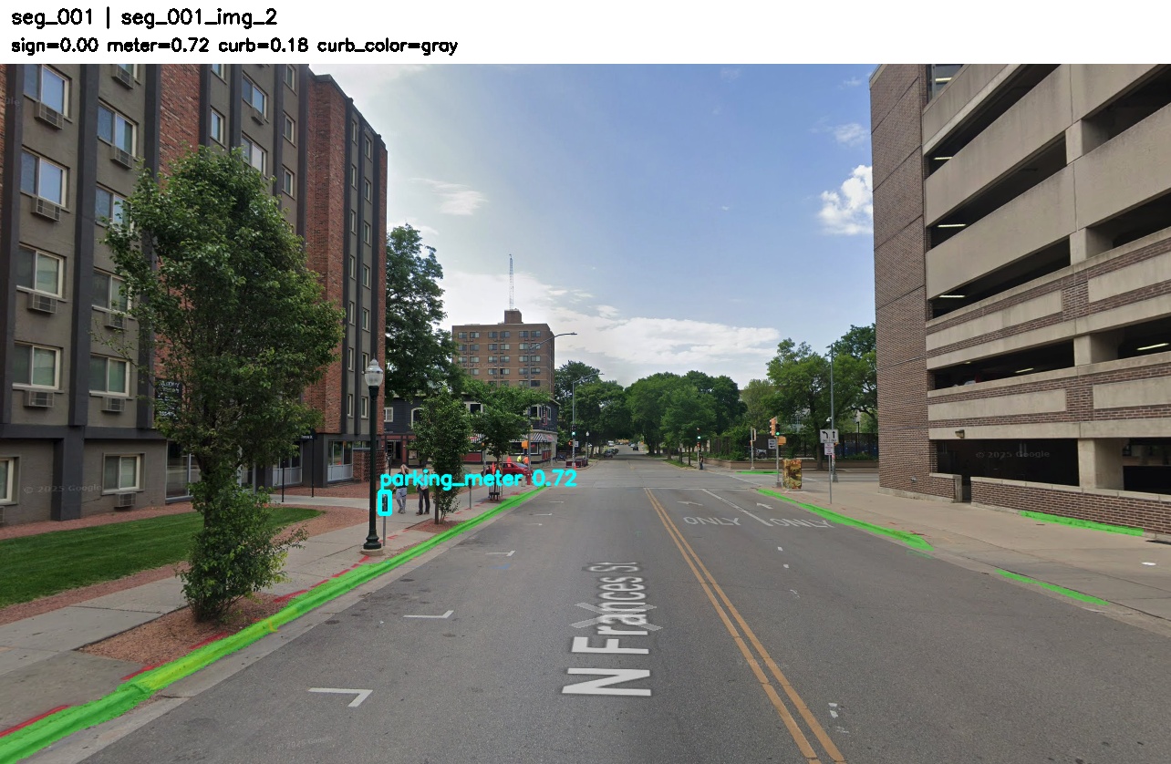
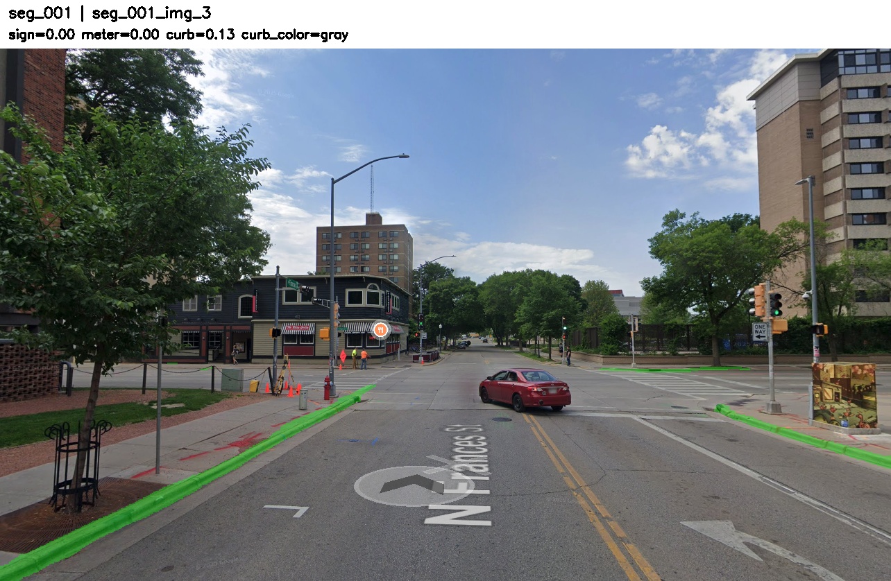
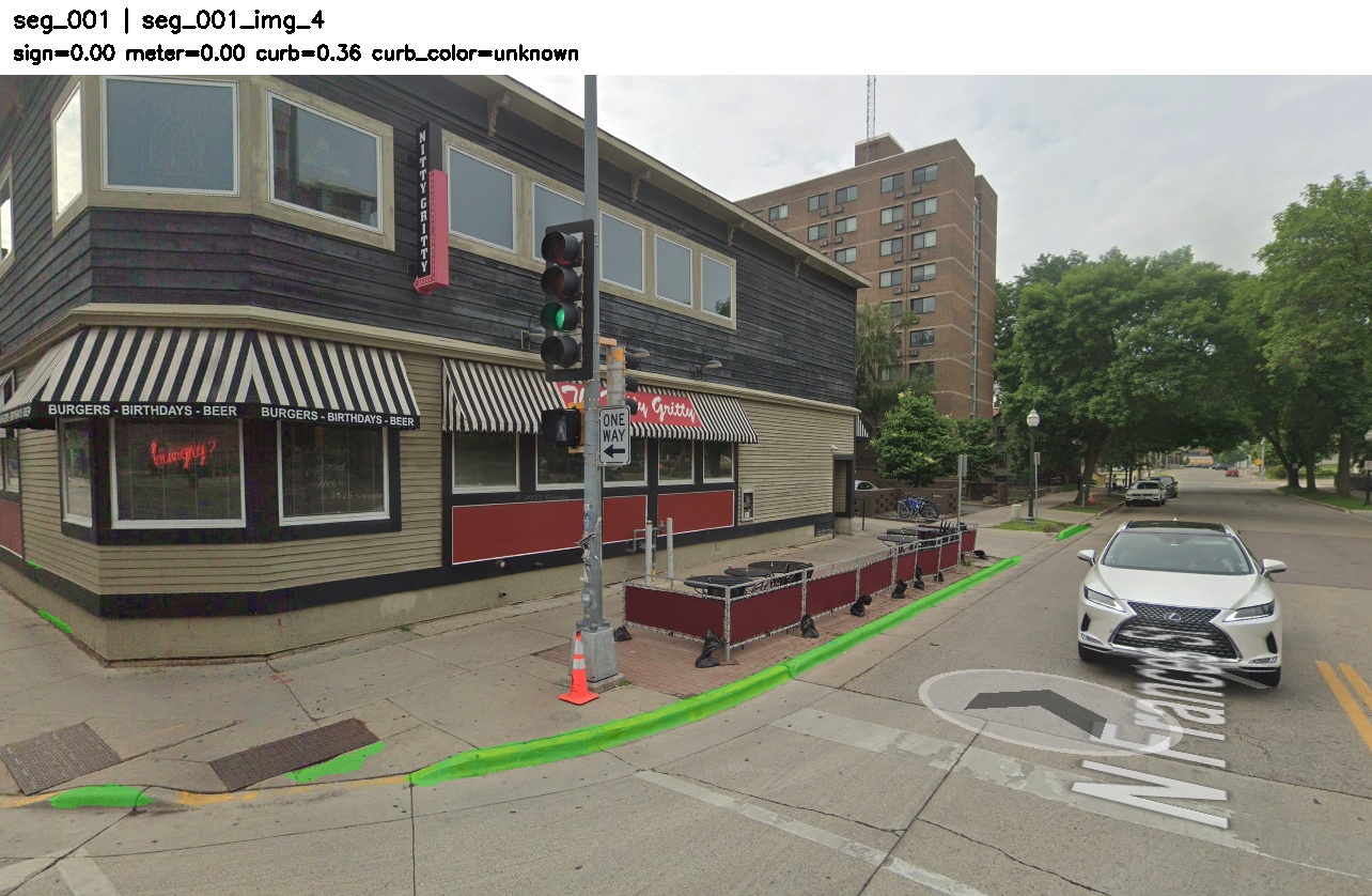
Manual segment seg_001. Meter-only segment — the sign detector does not fire, but the parking-meter cue is strong enough for segment-level aggregation to correctly classify it as positive.
4.2 seg_003 — curb-color borderline
Sign 0.148, Meter 0.000, Curb 0.407 → Combined 0.163. Just above the 0.15 threshold — appropriately uncertain. Curb color is meaningful but indirect; it should not dominate the final decision unless there is enough evidence. The low margin reflects uncertainty rather than overconfidence.
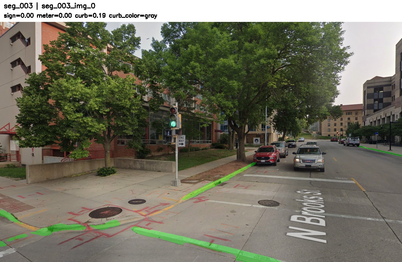
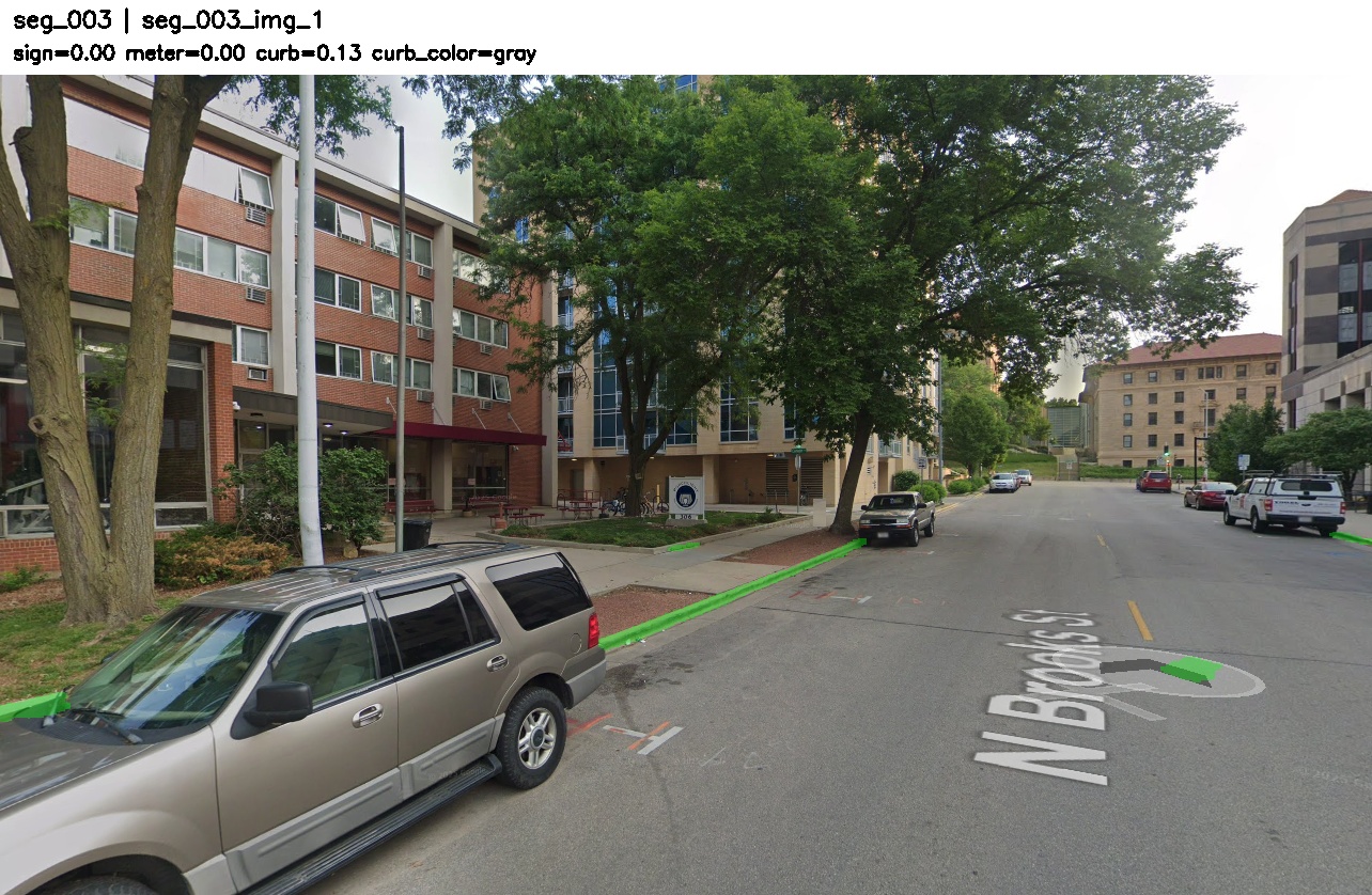
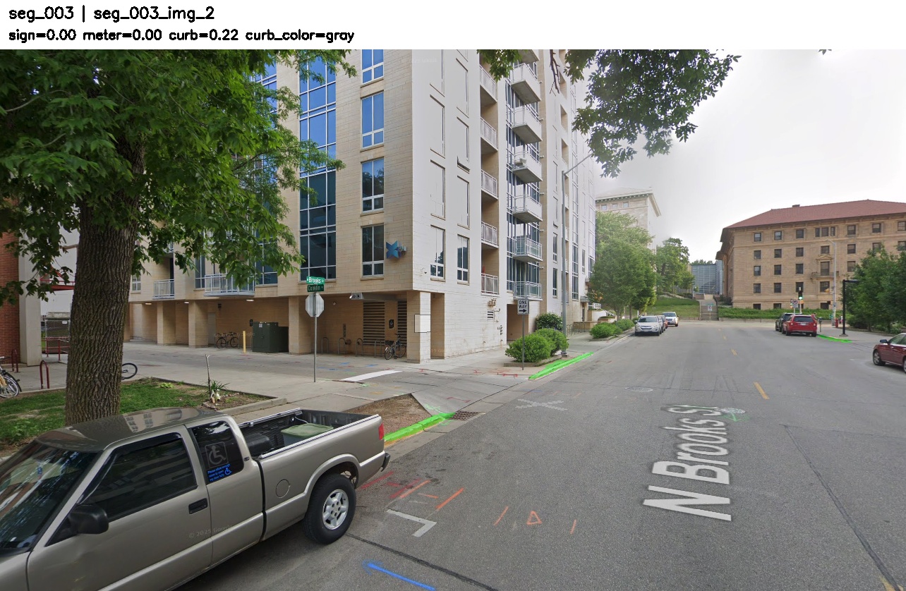
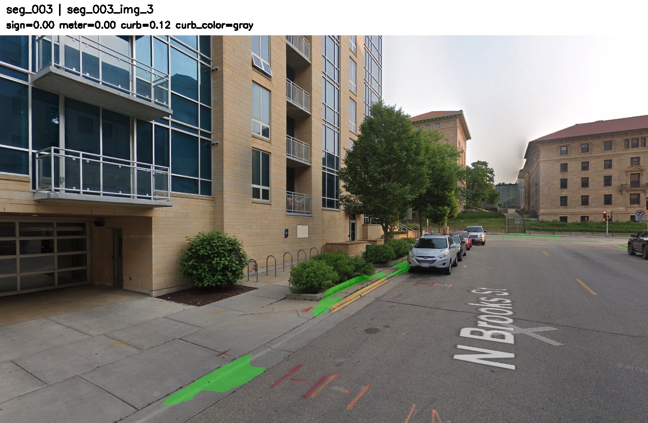
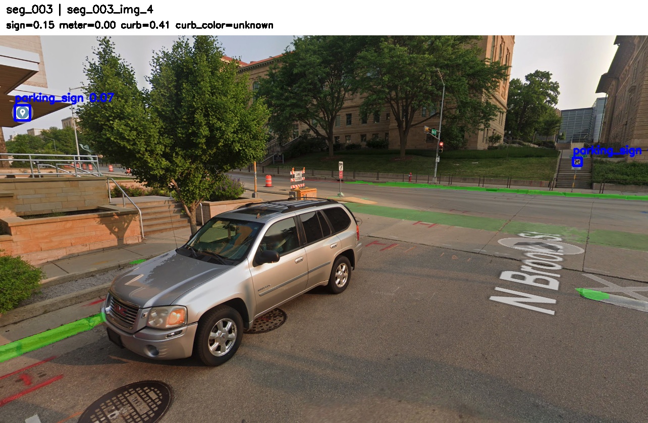
Manual segment seg_003. Curb-color-only example — a borderline but successful case. The low margin is appropriate because curb color is an indirect cue and is intentionally down-weighted.
4.3 seg_004 — complementary cue fusion
Sign 0.000, Meter 0.708, Curb 0.539 → Combined 0.425. The sign detector contributes nothing, but the meter and curb modules both produce useful signals. The segment is correctly recovered because aggregation combines auxiliary cues instead of requiring a sign detection.
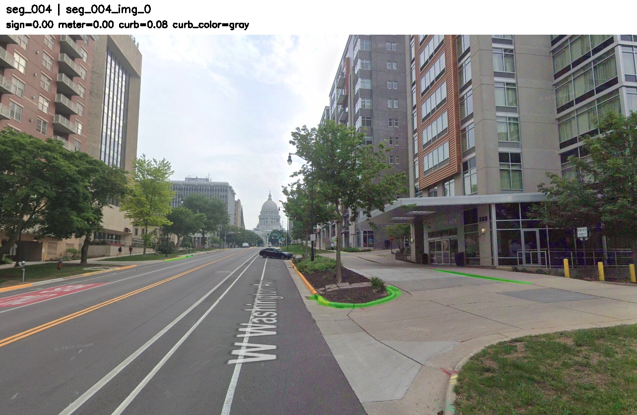
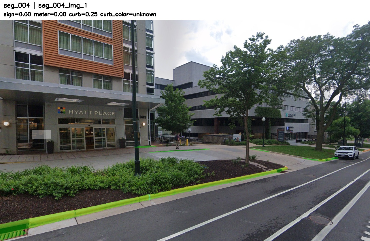
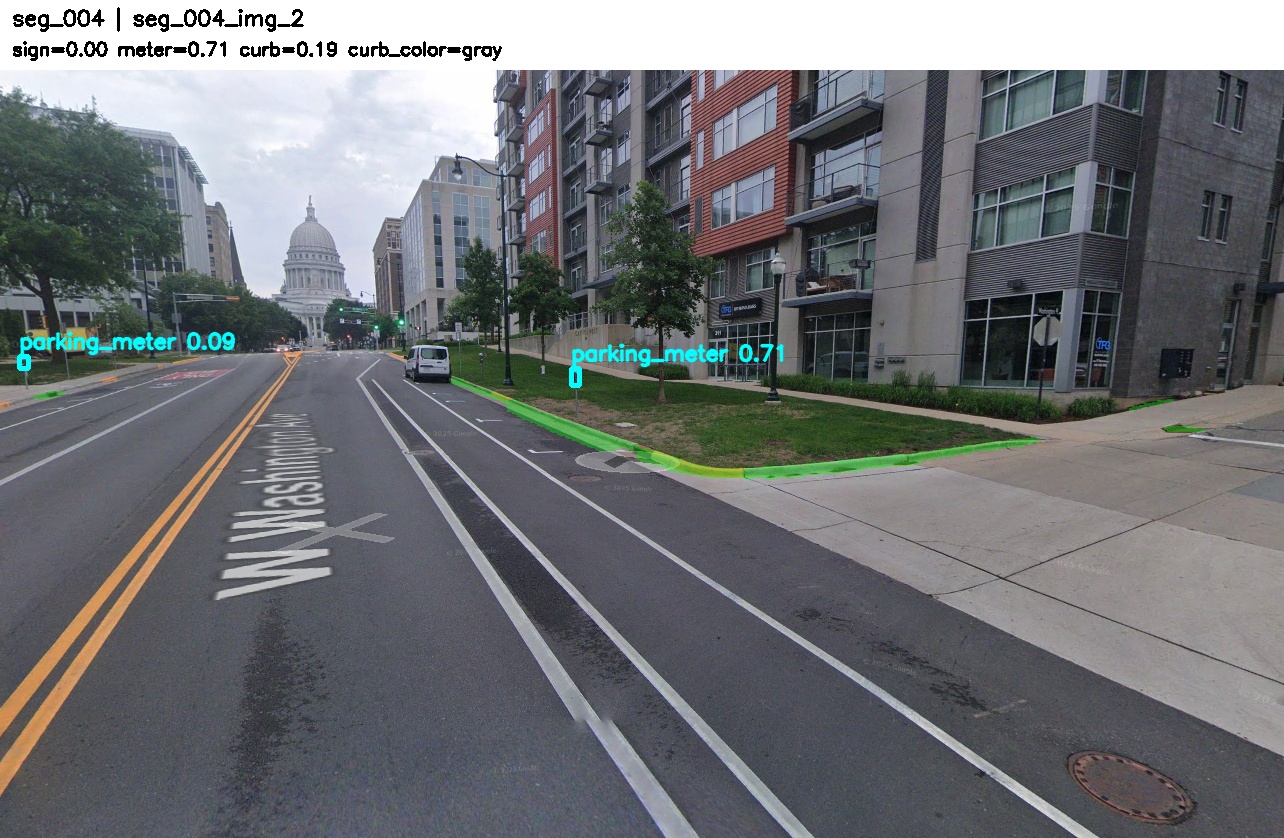
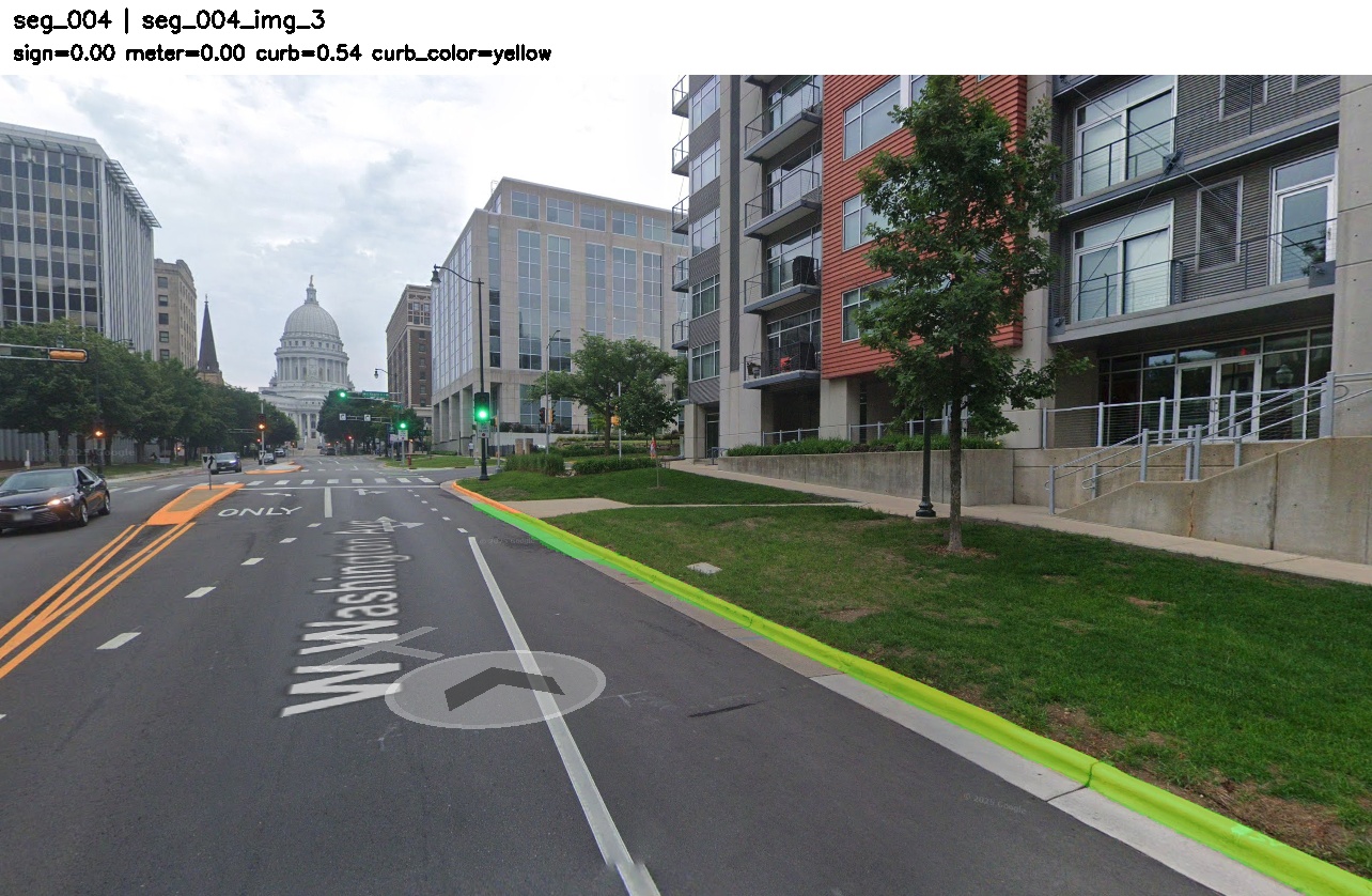
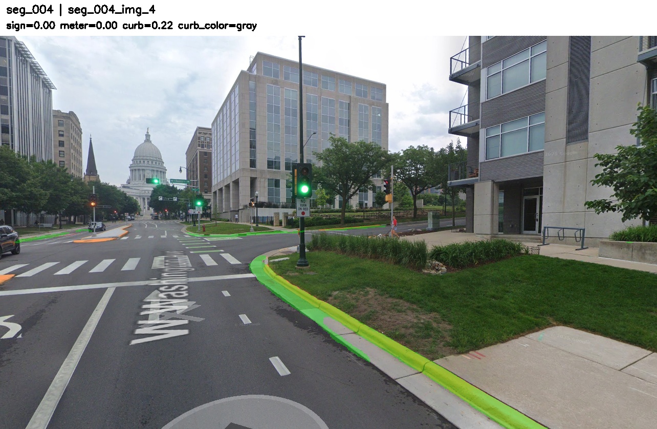
Manual segment seg_004. Combines meter and curb-color evidence. The sign detector contributes no signal, but aggregation succeeds via complementary auxiliary cues.
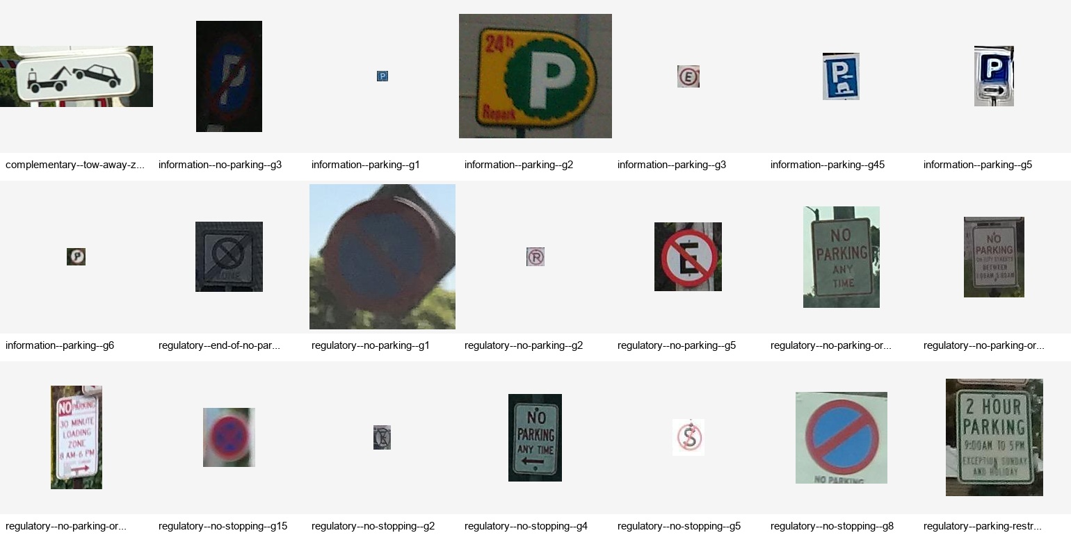
4.4 seg_005 — out-of-distribution failure
All cues near zero (combined 0.037). At first this looked like an image-quality issue, but closer inspection shows a more meaningful failure mode: the visible sign is outside the detector's training distribution. The system was trained on mapped MTSD parking-regulation signs, but the visible sign resembles a non-standard storefront or local sign. With no view containing a sign matching the trained detector's visual vocabulary, and no strong meter or curb backup cues, aggregation cannot recover the segment. Aggregation can compensate for sparse visibility, but it cannot compensate for a detector that lacks the relevant visual concept.
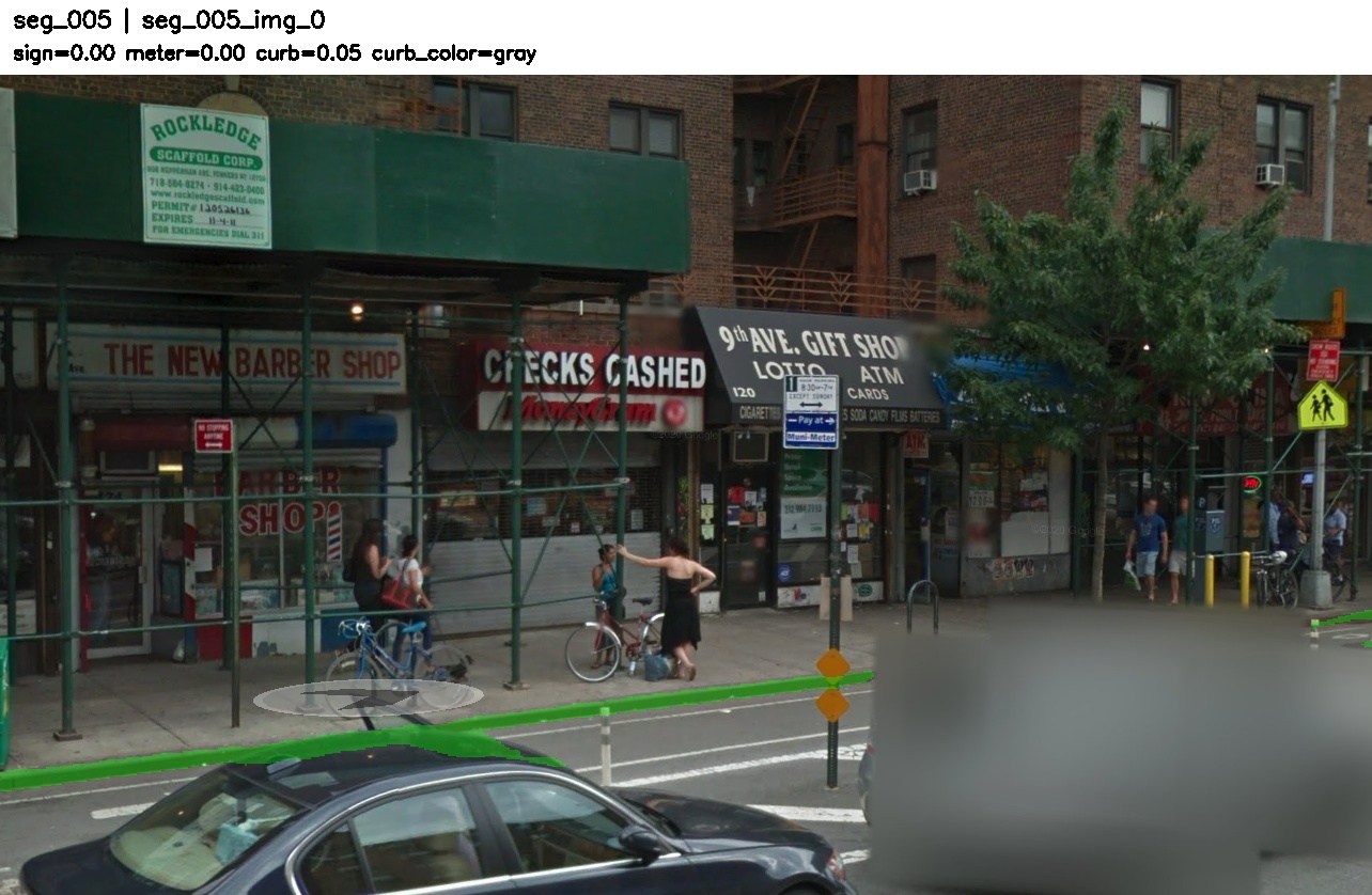
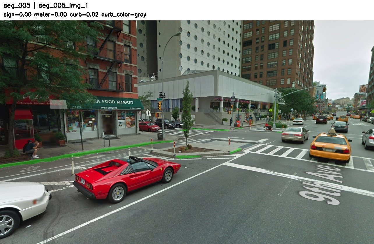
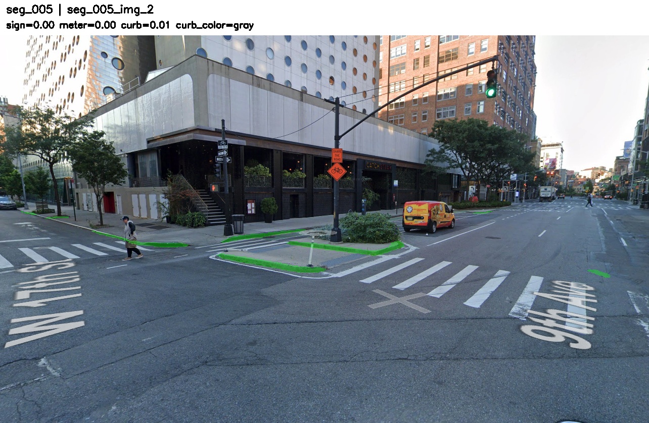
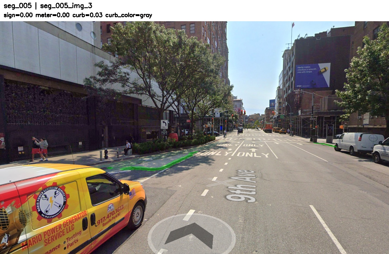
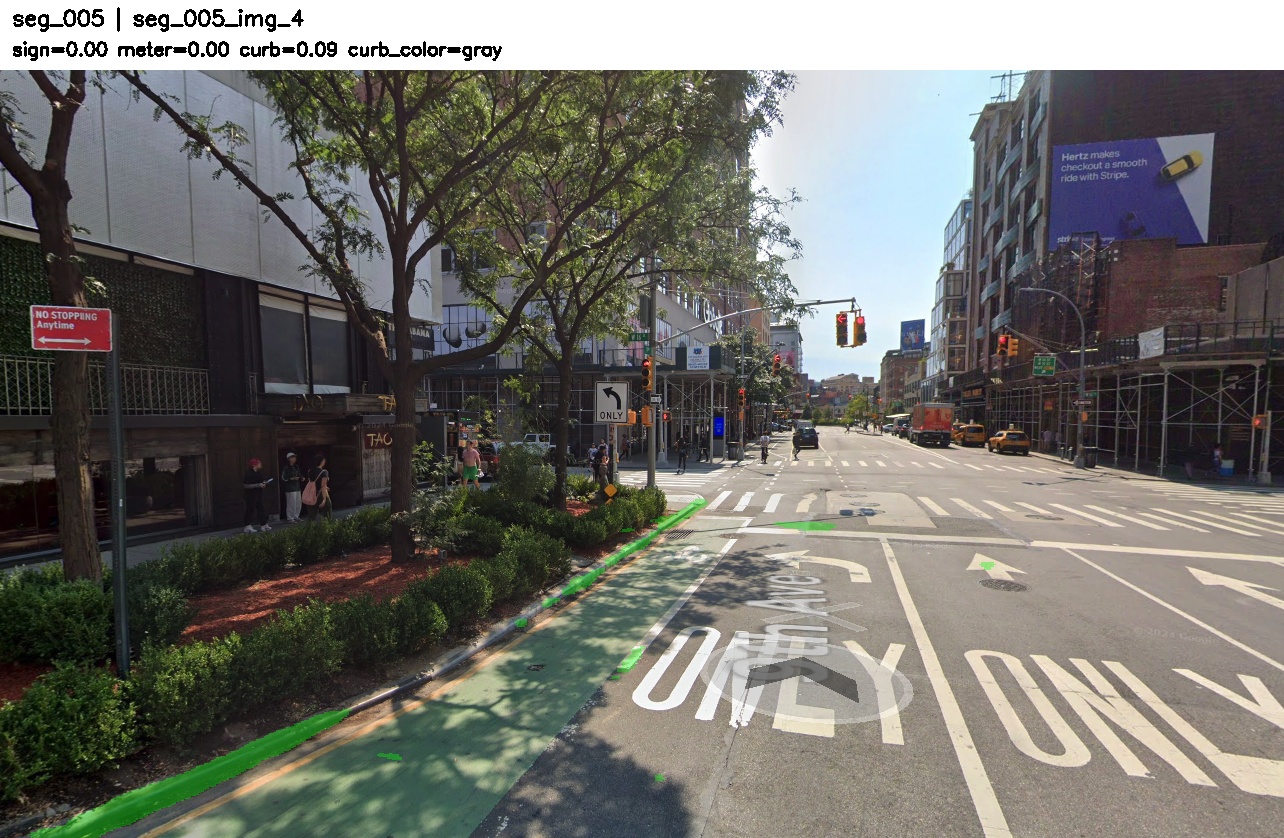
Manual segment seg_005. The visible sign is outside the training distribution, and there are no strong auxiliary cues. Aggregation cannot recover missing visual concepts.
4.5 Additional segments
Annotated views for the other two manual segments (seg_000 and seg_002).
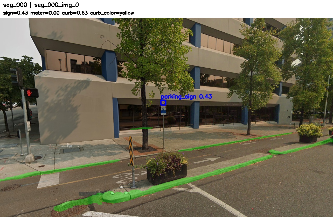
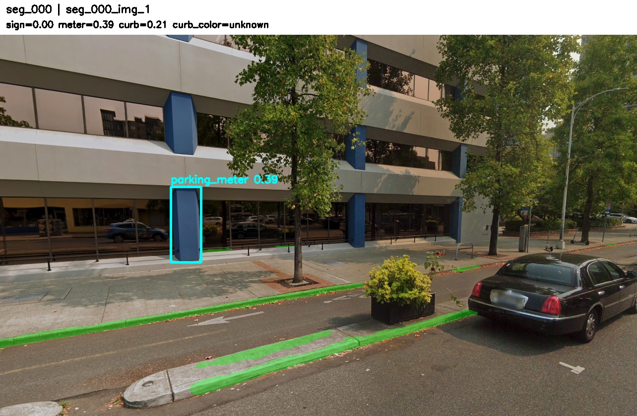
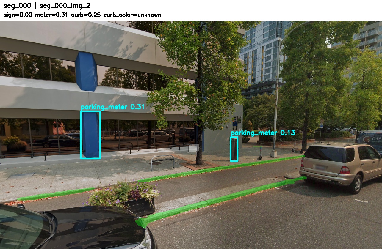
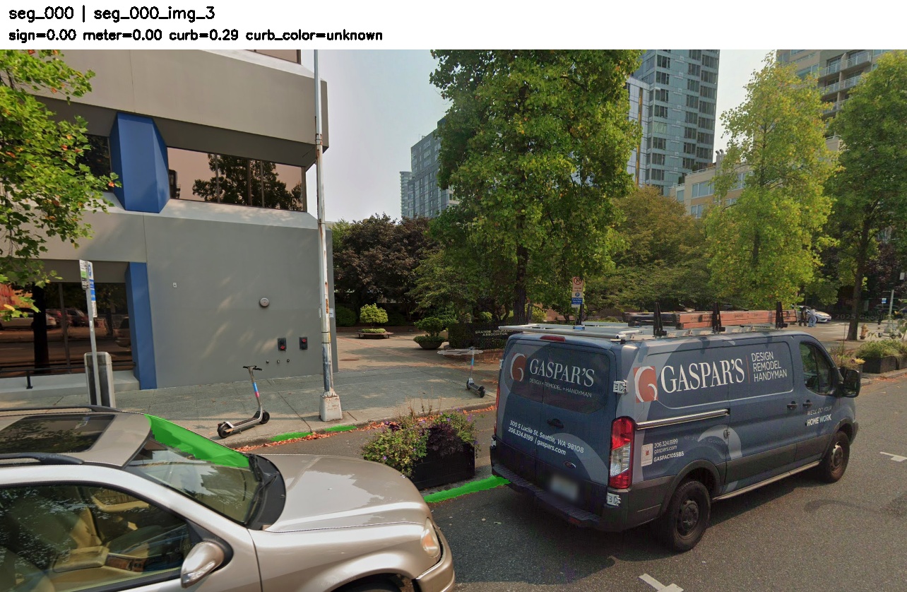
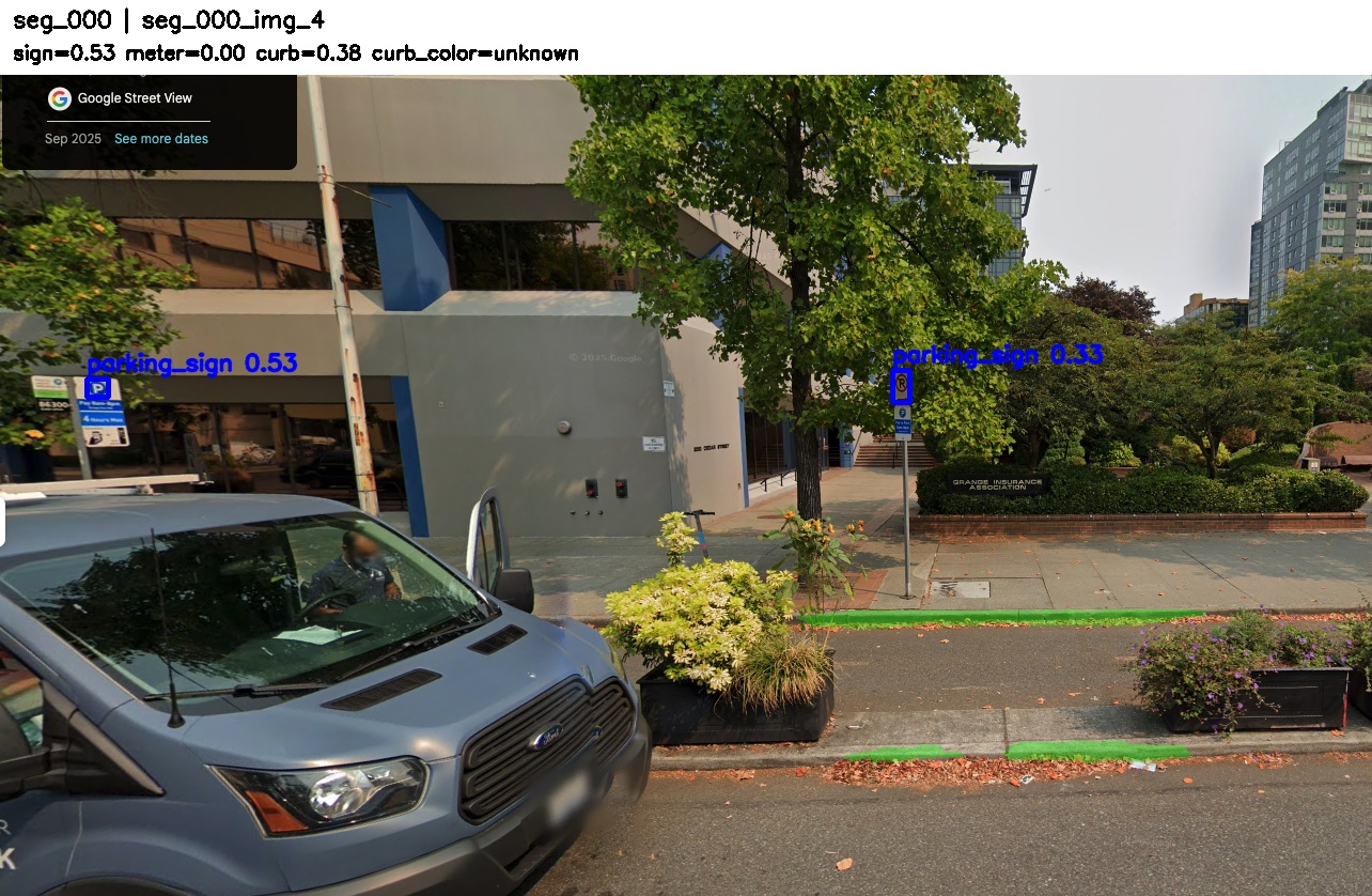
seg_000 — sign-only positive (single-image baseline also succeeds)
Sign 0.529, Meter 0.394, Curb 0.634 →
Combined 0.529. Multiple parking signs visible
across the five views. This tests whether aggregation increases
confidence when the sign detector already has evidence.
Note: The building pillar detected as a meter in view 2,
which is a common failure mode for the parking-meter detector and
a good example of why meter evidence should be down-weighted in
aggregation.
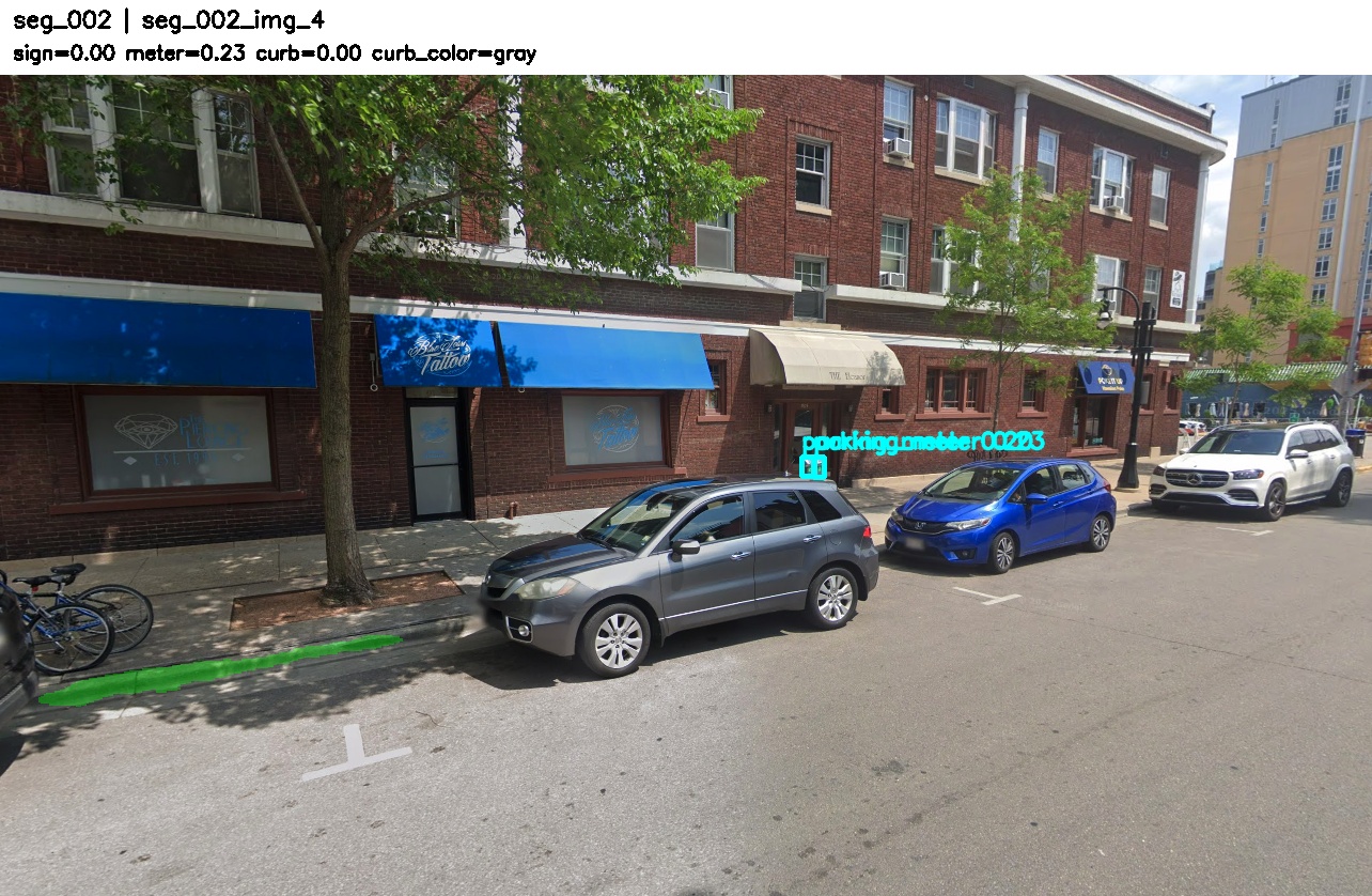
seg_002 — mixed-cue segment
Sign 0.395, Meter 0.227, Curb 0.426 → Combined 0.395. Mixed-cue segment containing parking meter, parking-sign evidence, and yellow curb color. Tests whether heterogeneous cues support the same segment-level decision.